Particle filters for continuous-time jump models in tracking applications

Christophe Andrieu & Dan Crisan, Editors DOI: 10.1051/proc:071907

PARTICLE FILTERS FOR CONTINUOUS-TIME JUMP MODELS IN TRACKING

APPLICATIONS

Simon Godsill

Abstract. In this article we summarise recent work in modelling and estimation of continuous-time jump models for application in tracking scenarios. The models are constructed such that random jumps occur in the driving function (typically the applied force on an object being tracked) at random times, and in general asynchronously with the observation times. The sojourn times between jumps are modelled as general distributions (here gamma or shifted gamma), and hence we are in the class of semi-Markov models, since the arrival times do not form a Poisson point process (see [21] for an overview of such models in the tracking setting). In contrast with other such models in the tracking literature we allow a fully continuous random set of manoeuvre parameters, rather than a discrete set of switching models, and deterministic paths during the sojourns, obeying a set of nonlinear kinematic equations for point mass motion, thus modelling the path of the object in a smooth and parsimonious fashion. These models are aimed at capturing the highly random manoeuvres of real objects in a simple way. Estimation is carried out using a Variable Rate Particle Filter (VRPF) that parameterises the model explicitly in terms of the jump times and their parameters [12, 13]. Extensions to the models and algorithms are also presented that allow for a diffusion component of the model, which captures continuous random disturbances to the object in addition to jumps. These are illustrated in a 3-dimensional linear Gaussian setting where the entire path, except for jump times, may be marginalised, hence making a more efficient and effective particle filter.

Introduction

In this paper we give a brief overview of recent work in tracking of highly manoeuvrable objects by the use of nonlinear jump processes and particle filters. The models developed are expressed in a natural intrinsic coordinate system which, it is postulated, represent realistic conditions more accurately (see [21] for evidence to back up this claim). New models and algorithms are presented for linear jump processes that also contain a Brownian driving component, and a fully Rao-Blackwellised particle filtering implementation is demonstrated for this setup. Initial proof-of-principle results are given for simulated trajectories.

∗_{The work of the author is partially funded by the EPSRC project Bayesian Inference for Continuous Time Diffusions, and}

by the UK’s Data and Information Fusion Defence Technology Centre 1 _{Signal Processing and Communications Group}

University of Cambridge

c

EDP Sciences, SMAI 2007

1.

Models - General Nonlinear Case

1.1.

Dynamical models

The class of models we consider initially comprises continuous-time trajectories having piecewise deterministic sections. The type of models proposed fits closely with the general class of piecewise deterministic processes, see [5], although we do not need to restrict to the Markovian case. In our models thekth section,k= 0,1, ...,

is parameterised by a time τk at which the section commences (τk > τk−1 > ...), and the parameters of the manoeuvreθk. A Markovian update on thekscale is defined for the combinedkth statexk = [θk, τk]:

x_k ∼f(x_k|x_k−1) =f_θ(θ_k|θ_k−1, τ_k, τ_k−1)f_τ(τ_k|θ_k−1, τ_k−1). (1)

The distributionfτ(τk|θk−1, τk−1) is quite general, subject to the constraintτk > τk−1, although we do constrain ourselves tofinite activityprocesses, i.e. those having a finite number of manoeuvre pointsτk in any finite time interval. We have typically used gamma, or shifted gamma, distributions for the inter-arrival times. Note that the parameters of the time distributions can explicitly depend on the manoeuvre parameters θk, and could themselves be made non-Markovian if required.

Having defined a skeleton for the process in this way in terms of a countable collection of states{x_k}∞_k=0, the continuous-time path of the process is defined as a deterministic function of these states. In general for models of this type the path could be a function of several neighbouring state variables, see [12, 13]. Here however we restrict ourselves to causal constructions in which the path at any timet≥τ₀depends only upon the two closest state points, N_t={k, k−1;τ_k−1 < t ≤τ_k}. Note that the underlying model here is a type of Marked point process, and hence the inference schemes proposed are for filtering of marked point process dynamical models, see [5, 6, 19] for example.

1.1.1. Example: Intrinsic Coordinates Motion Model [13]

To give a specific example, we construct the state variableθ_k for an object undergoing planar motion, subject to applied forcesT_T,k(tangentially to motion) andT_P,k (perpendicular to the motion), as

θk = [TT,k, TP,k, v(τk), ψ(τk), z(τk)]

where v(τ_k) is the speed at time τ_k, ψ(τ_k) is the heading angle relative to a fixed coordinate axis, and z(τ_k) is the Cartesian position of the object in the fixed Cartesian coordinate frame. This model is distinct from others in the area in that forces are applied relative to the body frame of the object, which is regarded as a more realistic model for motion of objects under self-forcing [21]. These models are however avoided in standard settings owing to the high degree of nonlinearity involved. In the particle filter implementation this is not an issue and we may go for greater realism. The kinematic equations for the object between timesτ_k andτ_k+1 are then obtained from standard considerations as

T_T,k=λds dt +m

d2s

dt2, TP,k=m ds dt

dψ

dt, τk ≤t < τk+1

wheres(t) is the total distance moved along the path from time 0. The parametersmandλdenote the mass of the object and the linear coefficient of resistance, respectively. Note that a linear resistance model is unrealistic for many scenarios, but has been found to be a reasonable approximation for the trajectories that we have so far encountered. Current research is investigating extensions that model a more realisticsquare law effect in the resistance, for which closed form solutions to the differential equation also exist. The model as posed above falls within the general class ofcurvilinear models [21], which are some of the most powerful generic models1of target motion currently available.

1_{By ‘generic’ we mean that the kinematics are not obtained from a direct modelling of the dynamics of a particular aircraft or}

In order to obtain the interpolated value of the pathz(t),τ_k−1≤t < τ_k, the kinematic equations are solved as standard coupled differential equations. The tangential equation is readily integrated from timeτ_ktoτ_k+τ to give the speedv(t) along the path at timet=τk+ ∆τ:

v(τ_k+ ∆τ) = 1

λ

T_T,k−(T_T,k−λv(τ_k))e−∆τλ/m

(2)

and the distance moved along along the path:

s(τk+ ∆τ) =s(τk) +∆τ

λ TT,k+ m

λ2(TT,k−λv(τk))(e

−∆τλ/m_{−1) (3)}

Then using the above expression for the speedv(t), the perpendicular equation is rearranged and integrated to give:

dψ dt =

T_P,k

mv(t), τk ≤tτk+1, v(t)= 0

ψ(τ_k+ ∆τ) =ψ(τ_k) +

_τk+∆τ

τk

T_P,kdt mv(t)

=ψ(τ_k) +T_P,k/T_T,k

∆τ λ/m−log v(τk)

v(τ_k+ ∆τ)

(4)

The results thus far are exact and in closed form, subject to the assumption that the forcing is constant between time pointsτkandτk+1. To determine the Cartesian positionz(t) = [x(t) y(t)]T of the object, however, appears to require a numerical integration procedure2. We achieve this by a simple Euler approximation on a fine time grid, calculating the changes inx−and y−coordinates over a time intervalδtas:

δx≈v(t) cos(ψ(t))δt, δy≈v(t) sin(ψ(t))δt, z(t+δt)≈z(t) + [δx, δy]T (5)

The model is then completed by assigning a probability distribution to the thrust parametersTT,k andTP,k. We have used independent Gaussian distributions for these, although a correlated Gaussian may also have useful properties (small forward thrust might imply small sideways thrust, for example).

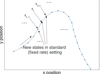
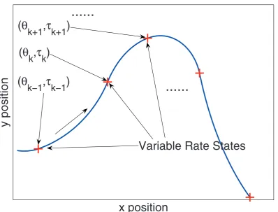
See Figs. 1 and 2 for simulated data from our dynamical model, comparing the more standard fixed rate setup (jumps arrive at regularly spaced time points) with the variable rate setup described here.

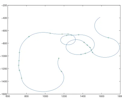
An example trajectory from the model is shown in Fig. 3, showing its clear ability to generate elaborate manoeuvres containing persistent turns of various types.

1.2.

Observation Models

The variable rate dynamical models are then linked with an observation process, whose arrival times are not chosen by us in this application. For convenience assume regularly spaced data at timest = 0,1,2.... The likelihood is then specified in terms of the interpolated dataz_t:

yt∼g(yt|x0:∞) =g(yt|zt).

whereg() is some known probability distribution for measurements given the path of the process at timet. The distribution g() is determined by the sensor characteristics. In standard tracking for radar, sonar, etc., the sensor is characterised by false alarms as well as missed detections, combining to give a point process of some kind. Similar features occur in video tracking when tracking is based on point features extracted from the raw image data.

2_{Under the simpler model whereλ= 0, i.e. there is no resistance force, the Cartesian position can also be obtained in closed}

x position

y position

x position

y position

x position

y position

...

New states in standard

(fixed rate) setting

x

t

x

t−1

x

t+1

...

...

...

Figure 1. _{Standard (fixed-rate) state sequence}

1.2.1. Example: Poisson Measurement Models [9, 10]

In this model a nonhomogeneous spatial Poisson point process is assumed as the model for both object-originating measurements and false-alarm (‘clutter’) measurements. In this way certain classical problems with data association [1] are bypassed, since the union property of two independent Poisson processes leads straightforwardly to a third Poisson process with well-defined intensity function. In this model the number of measurements from each target at each time point are assumed drawn randomly from a Poisson distribution having meanλT. Each such target measurement, say y, is assumed drawn from a sensor distributionpT(y|z) which is typically centered on the target statez, and may model the spatial extent and shape of the object/group (time index omitted for simplicity). Random clutter measurements are also included, whose number is again a Poisson random variable having mean λC and uniform or non-uniform spatial distribution pC(y). A useful consequence of this model is that the resulting random set of target and clutter measurements is also a Poisson point process having mean number of pointsλ_T +λ_C and distribution of individual points given by

(λ_Tp_T(y|z) +λ_Cp_C(y))

x position

y position

(

θ

k

,

τ

k

)

(

θ

k+1

,

τ

k+1

)

(

θ

k−1

,

τ

k−1

)

Variable Rate States

...

...

Figure 2. Variable rate state sequence

(see e.g. [4, 16]). Hence one may immediately write down the likelihood function for the observation values

y_t= [y_1,t, ..., y_Mt,t] and their numberM_tas [9]

g(yt, Mt|zt) =exp(−(λT +λC))

M_t!

Mt

i=1

(λTpT(yi,t|zt) +λCpC(yi,t))

whereMtis the total number of target and clutter measurements at timet. This model thus avoids any explicit treatment of the data association problem inherent in many tracking scenarios, but can potentially handle very high clutter densities. The model is typically used for tracking of group or extended targets, where the target is expected to make a random number of returns from random scatterer positions, or randomly from different objects in the group. The target distributionp_T(y|z) can model the shape and extent of the group, and could itself have parameters that evolve over time. With small mean target detection number λ_T the models may also be used successfully for modelling of small or spatially concentrated targets that exhibit random multipath effects or occasional multiple returns.

600 800 1000 1200 1400 1600 1800 −1600

−1400 −1200 −1000 −800 −600 −400 −200

Figure 3. Example trajectory from dynamical model,t= 0, ...,400. Jump instants shown as ‘+’.

2.

Linear SDE Models and Rao-Blackwellisation

a new sojourn having high driving noise. Nevertheless, the generic structure of the resulting Rao-Blackwellised particle filter algorithm has much in common with ours presented here3.

Consider first a 1-dimensional motion. 2- or 3-dimensional motions will be obtained by cascading several one-dimensional processes. A basic 1-dimensional motion model takes the following form:

T_t=λz˙+mz¨

whereλ≥0 is a motion resistance term andm >0 is the mass of the object as before, and{T_t}is a stochastic forcing term. In this sectionz(t) is interpreted as the Cartesian displacement of the object from the origin. We now assume that the stochastic forcing function is comprised of Brownian motion plus pure jumps:

T_t=σ_zB_t+W_t

whereBtis Brownian motion andWtis a pure jump process constructed from a marked point process{τk, Jk}, where{τk}are jump arrival times and{Jk}are the corresponding jump sizes, respectively. Then,Wtis obtained from the point process in the following way,

W_t= τk≤t

J_k, τ_k≤t < τ_k+1

We will require shortly the increments of this process, which are given by:

dW_t= Jk, t=τk 0, otherwise

We will assume for now that the jump sizes{J_k}are independent and normally distributed,

Jk∼ N(µJ, σ2_J)

(there are interesting possible extensions of the algorithms to scale mixtures of normals by including a latent scale parameter along with each jump parameter [7, 11, 23]).Note that this type of model has been proposed in the finance area for the pricing of options [25, 20], although analyses in that area tend to rely on Poisson point process arrivals and univariate continuous time models.

Jump times are drawn from a finite activity process, i.e. finitely many jumps occur in finite time intervals almost surely (we will in fact ensure this by using a gamma or shifted gamma distribution for the inter-arrival time distribution for jumps).

We thus have a linear SDE, as follows

dz¨=−λ

m¨zdt+

1

mdTt

which is seen to be an Ornstein- ¨Uhlenbeck (OU) process in the acceleration ¨z. We now write this as a continuous-time state-space model,

dzt=Aztdt+hdTt where:

zt=

⎡ ⎣ zz˙t_t

¨

z_t

⎤

⎦, A=

⎡

⎣ 00 10 01 0 0 −_mλ

⎤

⎦ _h=

⎡ ⎣ 00

1 m

⎤ ⎦

3_{We thank Simon Maskell for helpful suggestions regarding the regeneration of variable rate states that lie beyond the current}

This linear model has a simple solution, starting at statezsat time s < t:

zt=eA(t−s)zs+

_t

s e

A(t−u)_hdT

u, t > s.

=eA(t−s)zs+

_t

s e

A(t−u)_hdW u+

_t

s e

A(t−u)_hσ zdBu

=eA(t−s)zs+

k:s<τk≤t

J_keA(t−τk)_h+

_t

s

eA(t−u)hσ_zdB_u

where the middle term in the last line arises as the integral of the increments in the pure jump component. Since the{J_k}are independent and Gaussian, and{B_u}is Brownian motion, the Markovian state transition density, conditional upon the jump times, is Gaussian and may be obtained directly. Calculations are relatively straightforward, but note thatAhas repeated eigenvalues at zero; hence some special consideration is required and matrix exponentials are performed directly using Taylor series expansions. Then we obtain

f(zt+δt|zt,{τk; t < τk ≤t+δt}) =N(µ_t+δt|t, C_t+δt|t) with

µ_t+δt|t=eAδtzt+ k:t<τk≤t+δt

µJeA(t+δt−τk)_h

C_t+δt|t=σ_J2

k:t<τk≤t+δt

eA(t+δt−τk)_hhT_eA(t+δt−τk)T _+σ2

z

_t

s e

A(t−u)_hhT_eA(t−u)T_du

Note again that this is in linear Gaussian form. When this is connected to a linear Gaussian observation model the system may thus be solved using linear Gaussian state-space theory, i.e. the Kalman filter. The jump times are not known, however, so these can be inferred using a marginalised, orRao-Blackwellised particle filter.

3.

Inference Using Particle Filters

3.1.

General Nonlinear Case

The processes described above are semi-Markov since the inter-arrival distribution for jumps is not exponential in general. Particle filter inference is thus performed directly in terms of sequential updating of the jump times and their parameters, which we term avariable rate particle filter [12, 13, 15]. We consider as state variable at time t the current neighbourhood of states xNt ={xk, xk−1;τk−1 < t≤τk}. The particle filter samples new

i.e. N_t+ = min{k;τk > t}. The term fτ(τk|, τ_k(i₋)₁, t−1 < τk ≤t) denotes the dynamical model truncated so thatt−1< τk ≤t. Algorithm 1 summarises the algorithm as it applies to a general nonlinear dynamical model and sensor distributiong().

3.2.

Linear Gaussian Case

In the special case that the dynamical model is linear and Gaussian, as in Section 2, and also the observation model, i.e.

y_t=G_tzt+vt, vt∼N(0, Cv),

the same basic filtering structure applies but now we only simulateτkand not the manoeuvre parameter variable

θk. Instead the path of the process is marginalised conditional on the jump times {τk} and we store at each time, for each particle, the sufficient statistics for the Gaussian distributed state variablezt:

p(z(ti)|y0:t−1, τ_0:(i_N)+

t ) =N(zt|µ

(i)

t|t−1, Ct(|it)−1)

where µ(_ti_|)_t−1and C_t(_|i_t)₋₁, the predictive means and covariance, are sequentially updated for each particle using Kalman filtering recursions [8, 2]. The weight function is then updated according to the modified formula:

w_t(i)(j)=w_t(₋i)(₁j)p(y_t|y_0:t−1, τ(i)(j)

0:N+

t )

The predictive density p(yt|y0:t−1, τ_0:N+

t ) is obtained from the prediction error decomposition of the Kalman

filter (see e.g. [18]), i.e.

p(y_t|y_0:t−1, τ_0:N+

t ) =N(yt|Gµt|t−1, GCt|t−1G

T_+C v)

4.

Examples

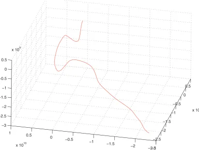
We present here brief examples for the tracking of an object in three dimensions using the linear Gaussian model of Section 2. For examples in the nonlinear models of Section 1.1.1, see our previous work [13, 9, 14, 15]. Consider a dynamical model according to Section 2 running independently in each of the three dimensions but coupled by idential {τ_k} values in all dimensions. The parameters of the models in each dimension are:

σ_z= 1000,µ_J= 0,σ_J= 50000. The jump process obeys a shifted gamma inter-arrival time, i.e.

τ_k−τ_k−1−τ_min∼G(α_τ, β_τ)

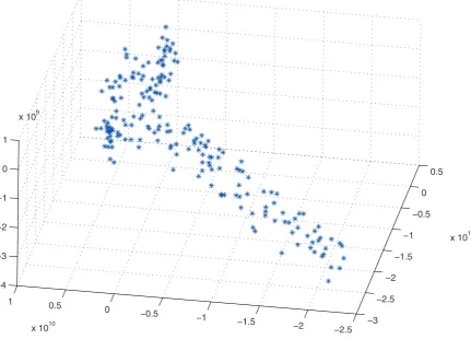
with τmin = 4, ατ = 0.5 and βτ = 4. The initial state in each dimension is centered at z0 = [0,0,0]T, with a Gaussian random perturbation of covariance 1002I and with initial jump time τ0 = 0. An example trajectory from such a process over a time interval [0,200) is given in Fig. 4. The total number of manoeuvres is 33 and it is clear that many manoeuvres have generated sharp turns and behaviour not characteristic of a standard linear Gaussian model (i.e. without jumps). Observations are generated from an additive Gaussian model in each dimension as

yt=zt+vt, vt∼N(0, σ2_v), σv = 5×108

Algorithm 1. _{Variable Rate Particle Filter}

.

Select number of offspringN_i for particlei,∀i∈ {1,2, ..., N}. fori= 1, ..., N do

Draw a binomial random variableN₀according to N_i trials, each with probability

α=

_∞

t fτ(τk|θk(i−)1, τk(i−)1)dτk

_∞

t−1fτ(τk|θk(i−)1, τk(i−)1)dτk

Choose how many particles require a new τ_k ∈[t−1, t).

N₁=N_i−N₀. N₁ is the number of particles for which a newτ_k ∈[t−1, t) should be generated. ResetN_i=N₁+ 1. Collapse particles for which no newτ_k is generated. Assign Nioffspring to each particle:

x(_Ni)(j)

t−1 =x (i)

Nt−1, w (i)(j) t−1 =

w(_t−i)₁

N_i , ∀j∈ {1, ..., Ni}.

Increase weighting for ‘collapsed’ particle:

w(_t−i)(₁N1+1)←N₀×w_t(i₋)(₁N1+1)

forj = 1, ..., N1do Sample paths that enforceτk ∈[t−1, t).

Setk=N_t+₋₁(i).

Sampleτ_k(i)(j)∼f_τ(τ_k|, τ_k(i₋)₁, t−1< τ_k ≤t) (use rejection sampling, or inverse cdf mapping). Sampleθ_k(i)(j)∼f_θ(θ_k|τ_k(i)(j),x(_ki₋)₁).

while(τ_k(i)(j)< t)do

k←k+ 1

Sample x(_ki)(j)∼f(x_k|x(_ki₋)(₁j)) end while

end for

forj = 1, ..., N_i do

Calculate interpolated state value,z(_ti)(j)from x(_Ni)(_tj).

Update weight:

w_t(i)(j)=w_t(₋i)(₁j)g(y_t|z(_ti)(j)) end for

end for

Restack the particles and weights from the replicates so that particle (i)(j) becomes particle (j+_i<iNi). Renormalise the weights such that

iNi

i=1 wt(i)= 1.

−3 −2.5

−2 −1.5

−1 −0.5

0 0.5

x 1010

−2.5 −2

−1.5 −1

−0.5 0

0.5 1

x 1010 −3

−2.5 −2 −1.5 −1 −0.5 0 0.5

x 109

Figure 4. Three-dimensional trajectory drawn from linear Gaussian jump model

5.

Discussion

We have reviewed existing methods for tracking using piecewise deterministic jump models, and presented new methods for linear Gaussian models having both jumps and a diffusion element. Interestingly it is possible to marginalise the entire path of the process in this setting, conditioned only on the arrival times of manoeuvres, allowing for a highly efficient Rao-Blackwellised particle implementation. Initial results look promising for the new methods but a full evaluation will be carried out in future work on the topic. The new models can potentially be linked in with nonlinear observation processes and data with clutter by partial Rao-Blackwellisation of the unobserved states (typically the velocities and accelerations) and by simulating data associations as part of the particle filtering process (see [27, 26] for examples of such ‘soft-gating’ procedures in other tracking models).

References

[1] Y. Bar-Shalom and T.E. Fortmann.Tracking and Data Association. Academic Press Inc.,U.S., 1988. [2] R. Chen and J. S. Liu. Mixture Kalman filter.J. Roy. Statist. Soc. Ser. B, 62(3):493–508, 2000.

−3 −2.5

−2 −1.5

−1 −0.5

0 0.5

x 1010

−2.5 −2

−1.5 −1

−0.5 0

0.5 1

x 1010 −4

−3 −2 −1 0 1

x 109

Figure 5. Data from three-dimensional trajectory

[4] D. Cox and V. Isham.Point Processes. Chapman & Hall, 1980.

[5] M. Davis. Piecewise-deterministic Markov processes: a general class of non-diffusion stochastic models (with discussion).J. Roy. Statist. Soc. Ser. B, (46), 1984.

[6] M.H.A. Davis.Markov Models and Optimization. Chapman and Hall, 1993.

[7] P. De Jong and N. Shephard. The simulation smoother for time series models.Biometrika, 82(2):339–350, 1995.

[8] A. Doucet, S. Godsill, and C. Andrieu. On sequential Monte-Carlo sampling methods for Bayesian filtering. Stat. Comput., 10:197–208, 2000.

[9] K. Gilholm, S.J. Godsill, S. Maskell, and D. Salmond. Poisson models for extended target and group tracking. InProc. SPIE: Signal and Data Processing of Small Targets, 2005.

[10] K. Gilholm and D. Salmond. A spatial distribution model for tracking extended objects. IEE Proc. on Radar, Sonar and Navigation, 152(5), 2005.

[11] S. J. Godsill. MCMC and EM-based methods for inference in heavy-tailed processes with alpha-stable innovations. InProc. IEEE Signal processing workshop on higher-order statistics, June 1999. Caesarea, Israel.

[12] S. J. Godsill and J. Vermaak. Models and algorithms for tracking using trans-dimensional sequential Monte Carlo. In Proc. IEEE Int. Conf. Acoust., Speech, Signal Process., 2004.

[13] S. J. Godsill and J. Vermaak. Variable rate particle filters for tracking applications. InProc. IEEE Stat. Sig. Proc., Bordeaux, July 2005.

−5 0

5

x 1010

−4 −2 0

2 x 1010 −5

0 5

x 109

−3 −2 −1 0 1

x 1010 −2.5

−2 −1.5 −1 −0.5 0 0.5

1x 10

10

−3 −2 −1 0 1

x 1010 −4

−3 −2 −1 0 1x 10

9

−3 −2 −1 0 1

x 1010 −4

−3 −2 −1 0 1x 10

9

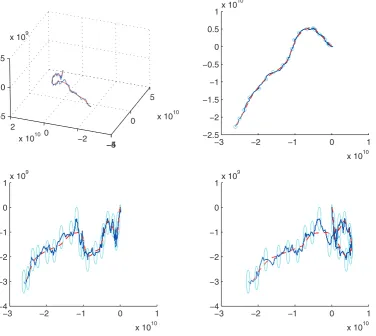
Figure 6. Posterior mean filtering estimates (true trajectory shown dotted). Top left: 3-d

plot. Top right: y vs. x with posterior confidence ellipses; bottom left: z vs. x with posterior confidence ellipses; bottom right: z vs. y with posterior confidence ellipses.

[15] S.J. Godsill, J. Vermaak, K-F. Ng, and J-F. Li. Models and algorithms for tracking of manoeuvring objects using variable rate particle filters.Proc. IEEE, April 2007. (To Appear).

[16] G. Grimmett and D. Stirzaker.Probability and Random Processes. Oxford University Press, third edition edition, 2001. [17] F. Gustafsson, F. Gunnarsson, N. Bergman, U. Forssell, J. Jansson, R. Karlsson, and P-J. Nordlund. Particle filters for

positioning, navigation and tracking.IEEE Transactions on Signal Processing, 50(2):425–437, February 2002. [18] A.C. Harvey.Forecasting, Structural Time Series Models and the Kalman Filter. Cambridge University Press, 1989. [19] M. Jacobsen.Point Process Theory and Applications. Marked Point and Piecewise Deterministic Processes. Birkhauser, 2006. [20] S.G. Kou. A jump-diffusion model for option pricing.Management Science, 48(8), August 2002.

[21] X.R. Li and V.P. Jilkov. Survey of maneuvring target tracking. part 1: Dynamic models.IEEE Trans. Aerospace and Electronic Systems, 39(4), 2003.

[22] J.S. Liu.Monte Carlo strategies in scientific computing. Berlin: Springer, 2001.

[23] M. Lombardi and S.J. Godsill. On-line Bayesian estimation of AR signals in symmetric alpha-stable noise.IEEE Trans. on Signal Processing, 2006.

[24] S. Maskell. Tracking manoevring targets and classification of their maneovrability.EURASIP Journal of Applied Signal Pro-cessing, 15, 2004.

20 22 24 26 28 30 32 34 36 38 40 0

0.02 0.04 0.06 0.08 0.1 0.12 0.14 0.16 0.18 0.2

Distribution of number of states

N_t+

p(N

t

+ |y

0:t

)

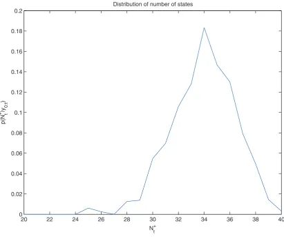
Figure 7. Estimate of probability of number of manoeuvres within time intervalt= 0, ...,200

(true value=33).

[26] J. Vermaak, S. Godsill, and P. Perez. Monte Carlo filtering for multi-target tracking and data association.IEEE Tr. Aerospace and Electronic Systems, 41(1):309–332, January 2005.