F. Coquel, M. Gutnic, P. Helluy, F. Lagouti`ere, C. Rohde, N. Seguin, Editors
TWO-SCALE CONVERGENCE
Emmanuel Fr´
enod
1Abstract. Those notes are the lecture notes of lectures given at Cemracs 2011 Summer School. I present here the classical results of Two-Scale Convergence Theory and an ap-plication to Homogenization of linear Singularly Perturbed Hyperbolic Partial Differential Equations.
R´esum´e. Ces notes constituent les notes du cours donn´e `a l’´ecole d’´et´e du Cemracs 2011. Je pr´esente les r´esultats classiques de la th´eorie de la convergence `a deux ´echelles et une application `a l’homog´en´eisation d’´equations aux d´eriv´ees partielles hyperboliques lin´eaires singuli`erement perturb´ees.
Contents
1. Introduction 2
1.1. On Two-Scale Convergence first statements 2
1.2. How Homogenization brought the concept 2
1.3. A remark concerning periodicity 10
1.4. A remark concerning weak-* convergence 10
2. Two-Scale Convergence - Definition and Results 14
2.1. Definitions 14
2.2. Link with Weak Convergence 15
2.3. Injection Lemma 16
2.4. Two-Scale Convergence criterion 19
2.5. Strong Two-Scale Convergence criterion 21
3. Application : Homogenization of linear Singularly Perturbed Hyperbolic Equations 23
3.1. Equation of interest and setting 23
3.2. A priori estimate 24
3.3. Weak Formulation with Oscillating Test Functions 24
3.4. Order 0 Homogenization - Constraint 24
3.5. Order 0 Homogenization - Equation forV 25 3.6. Order 1 Homogenization - Preparations: equation forU andu 26 3.7. Order 1 Homogenization - Strong Two-Scale convergence ofU 27
3.8. Order 1 Homogenization - FunctionW1 28
3.9. Order 1 Homogenization - A priori estimate and convergence 29
3.10. Order 1 Homogenization - Constraint 30
3.11. Order 1 Homogenization - Equation forV1 30
1 Universit´e Europ´eenne de Bretagne, Lab-STICC (UMR CNRS 3192), Universit´e de Bretagne-Sud, Centre Yves Coppens, Campus de Tohannic, F-56017, Vannes & Projet INRIA Calvi, Universit´e de Strasbourg, IRMA, 7 rue Ren´e Descartes, F-67084 Strasbourg Cedex, France
c
EDP Sciences, SMAI 2012
3.12. For the numerics 33
References 34
1.
Introduction
1.1.
On Two-Scale Convergence first statements
The concept of Two-Scale Convergence was introduced in two papers of Nguetseng [27, 28] in 1989. Then in 1992, Allaire [3] produced a synthetic and very readable proof of the result.
1.2.
How Homogenization brought the concept
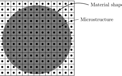
The concept of Two-Scale Convergence emerged from questions of Periodic Homogenization. Homogenization is a Mathematical Theory, or more precisely, an Asymptotic Analysis Theory that originates from Material Engineering, or more precisely, from understanding the way Constitutive Equation of composite material can be gotten from Constitutive Equation of each component of the concerned material and from their topological and geometrical distributions.
Microstructure Material shape
Figure 1.1. Composite material has a macroscopic shape and a microstructure. The ratio between the size of the microstructure and the size of the material isε.
In order to make the purpose clear, we first consider the simplest - but rich enough - example I know. (The explanation that follows does not aim to be mathematically rigorous. It clearly appeals to intuition and to non-rigorous vocabulary.)
Imagine that we want to get the temperature field within a composite material which is in thermal equilibrium, knowing the temperature on its boundary. Symbolically, as represented in Figure 1.1 (in a bi-dimensional setting), the composite material has a macroscopic shape at a macroscopic size. Within it, heterogeneities are more or less periodically distributed with a periodicity - or a characteristic size - which isεtimes smaller than its macroscopic size, whereεis a small parameter. This makes up what is usually called the microstructure of the composite material. Now, to achieve our goal, we contemplate the following Heat Equation
∇ ·haε(x,x ε)∇u
εi= 0 within the material,
uε given on the boundary of the material,
that is supposed to describe how the temperature uε is being split within the material from its distribution on the boundary. In this equation,aεstands for the Thermal Diffusion Coefficient (it is the ratio Thermal Conduction over Calorific Capacity times material Density), ∇and∇·stand for the gradient and divergence operators. (If a unidimensional material is considered,x=xlives inR, if a bi-dimensional material is considered, x= (x, y) lives inR2 and if a tridimensional material is
considered, x= (x, y, z) lives inR3.)
The fact that aεdepends on xandx/ε needs to be understood in the following sense. Variable xis the dimensionless position, meaning that when used to describe the material at its macroscopic scale, the needed variations of variable x are of the order of 1. Beside this, the dependence ofaε in x/εmodels the variation of the Thermal Diffusion at the microstructure scale. To illustrate this ability ofx/ε−dependence to describe variations at the microscopic scale, I show the graph of some kinds of functions in one and two dimensions. In Figure 1.2, is drawn the graph, between −πand
−4 −3 −2 −1 0 1 2 3 4 0.4
0.6 0.8 1 1.2 1.4 1.6 1.8
−4 −3 −2 −1 0 1 2 3 4 0.4
0.6 0.8 1 1.2 1.4 1.6 1.8
−4 −3 −2 −1 0 1 2 3 4 0.4
0.6 0.8 1 1.2 1.4 1.6 1.8
Figure 1.2. Graph of 1
2sin(x) + 1 +εcos( x
ε) forε= 1/20 (left), 1/40 (center) and 1/80 (right) between −πandπ.
π, of aε(x, x/ε) = (1/2) sin(x) + 1 +εcos(x/ε) forε= 1/20, 1/40 and 1/80. Those functions have a variation at the macroscopic scale, which is described by the piece (1/2) sin(x) + 1 and variations at much smaller scales, which are the microscopic variations. In this example, the microscopic variations can be qualified of being high frequency periodic oscillations with small amplitude. They are described by the term cos(x/ε) which needs to be multiplied by ε(explaining the presence of superscript εinaε) to insure amplitude of sizeεof those high frequency periodic oscillations. The
−4 −3 −2 −1 0 1 2 3 4 0
0.2 0.4 0.6 0.8 1 1.2 1.4 1.6 1.8 2
−4 −3 −2 −1 0 1 2 3 4 0
0.2 0.4 0.6 0.8 1 1.2 1.4 1.6 1.8 2
−4 −3 −2 −1 0 1 2 3 4 0
0.2 0.4 0.6 0.8 1 1.2 1.4 1.6 1.8 2
Figure 1.3. Graph of 12sin(x) + 1 +12cos(xε) for ε = 1/20 (left), 1/40 (center)
and 1/80 (right) between −πandπ.
piece (1/2) sin(x) + 1 and the variations at a smaller scale, making up the microscopic variations, are given by (1/2) cos(x/ε). (This term is not multiplied byε, bringing the uselessness of superscriptε inaε.) In this case the microscopic variations can be qualified of high frequency periodic oscillations with large amplitude or periodic Strong Oscillations. Figure 1.4 shows the ability of a function
−4 −3 −2 −1 0 1 2 3 4 −1
−0.8 −0.6 −0.4 −0.2 0 0.2 0.4 0.6 0.8 1
−4 −3 −2 −1 0 1 2 3 4 −1
−0.8 −0.6 −0.4 −0.2 0 0.2 0.4 0.6 0.8 1
−4 −3 −2 −1 0 1 2 3 4 −1
−0.8 −0.6 −0.4 −0.2 0 0.2 0.4 0.6 0.8 1
Figure 1.4. Graph of 1
2(sin(x) + 1) cos( x
ε) for ε= 1/20 (left), 1/40 (center) and 1/80 (right) between−πandπ.
depending onxandx/εto describe situations with microscopic variations which are with modulated amplitude - with regions where Oscillations are Strong and regions where they are not Strong. The drawn function is (1/2)(sin(x)+1) cos(x/ε). In this expression, the microscopic variations, which are high frequency periodic oscillations, are described by factor cos(x/ε) and the modulated amplitude is (1/2)(sin(x) + 1). Figure 1.5 shows function (1/2) cos(x) + 1 + (1/2)(sin(x) + 1) cos(x/ε) for always
−4 −3 −2 −1 0 1 2 3 4 −0.5
0 0.5 1 1.5 2 2.5
−4 −3 −2 −1 0 1 2 3 4 −0.5
0 0.5 1 1.5 2 2.5
−4 −3 −2 −1 0 1 2 3 4 −0.5
0 0.5 1 1.5 2 2.5
Figure 1.5. Graph of 12cos(x) + 1 +12(sin(x) + 1) cos(xε) forε= 1/20 (left), 1/40
(center) and 1/80 (right) between−πandπ.
the same values of ε. Those functions possesses both macroscopic scale variation and modulated amplitude high frequency oscillations as microscopic variations.
In every example above the microscopic scale variations are periodic. Yet, thex/ε−dependence may also describe microscopic scale variations that are not periodic. This is illustrated in figure 1.6 where function (1/10) sin(x/3) + 1 + (1/4) cos(x/ε) sin((π/4)x/ε) is drawn.
Despite the fact that, for visibility reasons, the chosen value ofεis not very small (1/20), figures 1.7 and 1.8 show bi-dimensional functions with periodic Strong Oscillations (figure 1.7) and modulated amplitude in one direction (figure 1.8).
ï10 ï8 ï6 ï4 ï2 0 2 4 6 8 10 0.7
0.8 0.9 1 1.1 1.2 1.3 1.4
ï10 ï8 ï6 ï4 ï2 0 2 4 6 8 10
0.7 0.8 0.9 1 1.1 1.2 1.3 1.4
ï10 ï8 ï6 ï4 ï2 0 2 4 6 8 10
0.7 0.8 0.9 1 1.1 1.2 1.3 1.4
Figure 1.6. Graph of 101 sin(x3) + 1 +14cos(xε) sin(π4xε) forε= 1/20 (top), 1/40
(center) and 1/80 (bottom) between−3πand 3π.
0
1
2
3
0 1 2 3 0 5 10 15
0
1
2
3
0 1 2 3 0 5 10 15
Figure 1.7. Graph ofx2+y2+12(sin(yε) + 1) + (sin(xε) + 1) (left) and ofx2+y2+
1 2(sin(
y
ε) + 1)(sin( x
ε) + 1) (right) forε= 1/20 on [0,3] 2.
It is practicable to introduce a variable (say ξ, which may beξ, (ξ, υ) or (ξ, υ, ζ), depending on the dimension number) which describes the variations at the microscopic scale. This consists in considering that aε in fact depends on two variables: aε(x,ξ) and that the coefficient in equation (1.1) is
aε(x,ξ= x
0
1
2
3
0 1
2 3
0 5 10 15
Figure 1.8. Graph ofx2+y2+ sin(2x)(sin(yε) + 1) + (sin(xε) + 1) forε= 1/20 on [0,3]2.
Applying this practicable trick to the examples involved in figures above, the following formulas are gotten:
aε(x, ξ) =1
2sin(x) + 1 +εcos(ξ), in the case of figure 1.2,
aε(x, ξ) =a(x, ξ) =1
2sin(x) + 1 + 1
2cos(ξ), in the case of figure 1.3,
aε(x, ξ) =a(x, ξ) =1
2(sin(x) + 1) cos(ξ), in the case of figure 1.4,
aε(x, ξ) =a(x, ξ) =1
2cos(x) + 1 + 1
2(sin(x) + 1) cos(ξ), in the case of figure 1.5,
aε(x, ξ) =a(x, ξ) = 1 10sin(
x 3) + 1 +
1
4cos(ξ) sin( π 4ξ),
aε(x, y, ξ, υ) =a(x, y, ξ, υ) =x2+y2+1
2(sin(υ+ 1) + (sin(ξ) + 1), and
aε(x, y, ξ, υ) =a(x, y, ξ, υ) =x2+y2+1
2(sin(υ) + 1)(sin(ξ) + 1)
in the case of figure 1.7, and,
aε(x, y, ξ, υ) =a(x, y, ξ, υ) =x2+y2+1
2(sin(υ) + 1)(sin(ξ) + 1), in the case of figure 1.8. (1.3)
Ifξ7→aε(x,ξ) is periodic, the microscopic scale variations are qualified of high frequency periodic oscillations.
Remark 1.1. Two-Scale Convergence is essentially designed to be used in the context of high fre-quency periodic oscillations.
an approximated solution of Partial Differential Equation (1.1). Since,xis a dimensionless variable, the domain on which (1.1) is set has a size which order of magnitude is 1. But, to get a reasonable result, we must choose a discretization step ∆xwhich is such that ∆x << ε. Otherwise, the effect of the microstructure is not taken into account, and the resulting computation has nothing to do with reality. Hence, if εis very small, meaning that the microstructure is much smaller than the macroscopic size, the computation can be very expensive and even not feasible. For instance, if we consider a tridimensional material, with ε = 10−3 then, with the constraint ∆x << ε, that we consider to be achieved with ∆x= 10−1ε, the order of magnitude of the number of degrees of freedom needed for the computation is (10·103)3 = 1012. This is quite expensive. Leading such a computation may not be completely unreasonable if we are interested in knowing the intimate distribution of the temperature at the microstructure scale, but in most of the situations the tiny variations at this scale have no interest. In those cases, it is highly unreasonable to lead such a heavy computation to get the result.
Hence, we would like to have on hand an equation, which does not explicitly involve any mi-crostructure, but which contains, or more precisely, which induces in its solution the average effect of the microstructure (which is described by the x/ε−dependence of aεin 1.1). Denoting symboli-cally this equation by
Hu= 0, (1.4)
involving an operator H, with the constraint that u is close to uε in some senses, we can expect to implement a numerical method to compute an approximated solution of (1.4) - which is also an approximation of uε - with a cost much smaller (because the constraint ∆x << ε is useless) than the one needed for the direct approximation of equation (1.1).
Homogenization Theory gathers a collection of methods that allows us to build operators H sat-isfying the required constraint.
The first Homogenization methods were set out by Engineers in the middle of the 1970s and then formalized by Mechanical Scientists. They are based on Asymptotic Expansion. Applying them in the case of equation (1.1) consists in writing
uε(x) =U(x,x
ε) +εU1(x, x ε) +ε
2U 2(x,
x
ε) +. . . , (1.5)
with functionsU(x,ξ),U1(x,ξ),U2(x,ξ), . . . periodic with respect toξ, in injecting this expansion in equation (1.1), in identifying and gathering terms in factor ofε−2,ε−1,ε0,ε,ε2, . . . and then in deducing a set of equations:
H−2U = 0, (1.6)
H−1U1=I(U), (1.7)
H0U2=I0(U, U1), (1.8)
. . . .
Then, if we want to get a rigorous mathematical justification of the process just described, we need to prove results like
u
ε
(x)−U(x,x ε)
?
→0, (1.9)
for a norm k k?to be determined, or in a weaker sense,
uε(x)−U(x,x ε)
*0. (1.10)
If we want to get justifications at higher orders, we need to prove convergence results like
uε(x)−U(x,x ε)
ε −U1(x, x ε)
→0, (1.11)
in some senses,
1
ε
1
ε
uε(x)−U(x,x ε)
−U1(x, x ε)
−U2(x, x ε)
→0, (1.12)
in some senses, and so on.
In the case of a Parabolic Partial Differential Equation like (1.1), with Dirichlet boundary condi-tions, convergence results of the kind of (1.9) can be brought out using the Maximum Principle and boundary estimates (see Bensoussan, Lions & Papanicolaou [5]).
In other cases, the way is less straightforward, and appeals to Oscillating Test Functions used within a Weak Formulation of the Partial Differential Equation. Passing to the limit using Compensated Compactness like results (see Tartar [36]) may give convergence results of the kind of (1.9) or (1.10). This method is called ”Energy Method” or ”Oscillating Test Function Method” and was designed by Tartar [35] in collaboration with Murat [26] (see also [5]). For mathematical justification, works of Engquist have also to be consulted, in particular [11].
The Weak Formulation with Oscillating Test Functions writes, in the case of equation (1.1),
Z
Material
∇ ·haε(x,x ε)∇u
ε(x)iϕ(x,x
ε)dx= 0, (1.13)
which yields, using the Stokes Formula,
Z
Material aε(x,x
ε)∇u
ε(x)· ∇hϕ(x,x ε)
i
dx=
Z
Boundary
Something, (1.14)
or
Z
Material aε(x,x
ε)∇u ε(x)
·
∇xϕ(x,
x ε) +
1 ε∇ξϕ(x,
x ε)
dx=
Z
Boundary
Something. (1.15)
In those integrals,∇uε converges generally in a weak sense only and this is the same for the other involved functions: aε(x,xε), ∇xϕ(x,xε) and ∇ξϕ(x,xε). It is well known that passing to the limit
in a product of two weak converging sequences of functions is a non-straightforward task. Hence, passing to the limit in (1.13), (1.14) or (1.15) is not so easy and consequently involves relatively sophisticated analytical methods (like Compensated Compactness results).
Two-Scale Convergence offers an efficient framework to pass to the limit in such terms, in the case when oscillations are periodic. It is certainly possible to infer that Two-Scale Convergence emerges from those kind of questioning. Yet, as it will be illustrated by the example treated in section 3, Two-Scale Convergence is much more than a method to justify Asymptotic Expansion: it is a constructive Homogenization Method very well adapted to Singularly Perturbed Hyperbolic Equations.
Two-Scale Convergence is a homogenization tool which is well adapted to situations involving periodicity. In the non periodic setting more refined tools are needed. I refer to the book of Tar-tar [38] for the descriptions of those methods. Among them,G-convergence (see Pankov [32]) is well adapted to problem involving Green Kernel, Γ-convergence (see Dal Maso [9] and Braides [7]) is a tool designed for homogenization of optimization problems. I also mention the very sophisticated H-measures of Tartar [37] and G´erard [24] that allow to tackle fine homogenization questions within the micro-local calculus framework.
Of course, we can try to provide an answer to questions of the same type as before in other field than composite material. For instance we can be interested in the time varying version of (1.1):
∂uε ∂t − ∇ ·
h
aε(x,x ε)∇u
εi= 0 within the material,
uε(t, .) given on the boundary of the material,
uε(0, .) given at initial time within the material,
(1.16)
where tstands for a dimensionless time and wherexhas the same meaning as in equation (1.1). We can also consider the following equations :
∂zε ∂t −
1 ε∇ ·
a(t,t ε,x)∇z
=1 ε∇ ·c(t,
t
ε,x), (1.17)
and
∂zε ∂t −
1 ε2∇ ·
a(t,t ε,x)∇z
= 1
ε2∇ ·c(t, t
ε,x), (1.18)
which are relevant models for the short-term and long-term dynamics of dunes on a seabed of a coastal ocean where tide is strong. In equation (1.17) and (1.18),zε=zε(t,x), wheretstands is the dimensionless time andxis the bi-dimensional dimensionless position variable, is the dimensionless seabed altitude at timetand in positionx.Those equations were widely studied in Faye, Fr´enod & Seck [12, 13].
We can also be interested in the following Vlasov equations :
∂fε
∂t +v· ∇xf
ε+ (E(x, t) +1
εv×B(x, t))· ∇vf
ε= 0, (1.19)
and
∂fε
∂t +vk· ∇xf ε+1
εv⊥· ∇xf
ε+ (E(x, t) +1
εv×B(x, t))· ∇vf
ε= 0, (1.20)
which are models involved in Tokamak Plasma physics. In those equations x ∈R3 stands for the
dimensionless position, v∈R3 for the dimensionless velocity andtfor the dimensionless time. The
Those two last equations involve neither oscillating coefficients nor any microstructure. Neverthe-less, the strong magnetic field induces in the solution high frequency periodic oscillations. Equations (1.19) or (1.20) can be cast into the following framework of a singularly perturbed convection equa-tion:
∂uε
∂t +a· ∇u ε+1
εb· ∇u
ε= 0, x∈
Rd, t >0, (1.21)
by setting, in the case of (1.19),
a(x,v, t) =
v E(t,x)
andb(x,v) =
0 v×B(t,x)
, (1.22)
and, in the case of (1.20),
a(x,v, t) =
vk E(t,x)
andb(x,v) =
v⊥
v×B(t,x)
. (1.23)
Equation of this type are studied in Fr´enod & Sonnendr¨ucker [20–22], Fr´enod & Watbled [23], Fr´enod, Raviart & Sonnendr¨ucker [18], Fr´enod [14, 15], Fr´enod & Hamdache [16] Ailliot, Fr´enod & Monbet [1, 2], Fr´enod, Mouton & Sonnendr¨ucker [17] and Fr´enod, Salvarani & Sonnendr¨ucker [19] .
1.3.
A remark concerning periodicity
Two-Scale Convergence is well-adapted to the framework of high frequency periodic oscillations (or to cases that can be brought to this framework by an adequate transformation). But, it essentially does not work in non-periodic cases. Even in the case of oscillations with a period depending on the variable describing the macroscopic variation, it does not work. Many questions linked with non-periodic homogenization are essentially open.
1.4.
A remark concerning weak-* convergence
Here, I give the proof of two important and representative results. They concern the characteri-zation of the weak limit of functions with high frequency periodic oscillations.
I will denote, for p= 1, . . . ,∞, byLp(
R) the space of functions defined almost everywhere onR
such that theirp-th power is Lebesgue integrable, byLp#(R) the space of functions being inLp(
R) and
periodic of period 1, byC0
#(R) the space of functions being continuous overRand periodic of period 1, byC∞(
R) the space of functions being infinitely derivable overRand byD(R) the space of functions
being inC∞(
R) and compactly supported. Finally, we denote byLp(R;C#0(R)) the Lebesgue space of Bochner integrable functions mappingRtoC0
#(R). This space can be characterized as the space of functions mappingRtoC#0(R) such that thep-th power of their norm is Lebesgue integrable ifp <∞ and such that their norm is essentially bounded ifp=∞. (I refer the reader to Bochner [6], Diestel & Uhl [10], Yosida [39] and Schwartz [34] for a precise and thoroughly description of Integration Theory, specifically for functions with values in Banach spaces.)
The first result , which is often referred to as the ”Riemann-Lebesgue Lemma”, gives the asymp-totic behavior, with respect to weak topology, of a periodic function applied in ξ=x/ε.
Lemma 1.2. Let ψ∈L∞#(R). Defining [ψ]ε by[ψ]ε(x) =ψ(x
ε), then
[ψ]ε*
Z 1
0
Remark 1.3. Convergence (1.24) means that for any functionφ∈L1(
R),
Z
R
[ψ]ε(x)φ(x)dx→
Z 1
0
ψ(ξ)dξ
Z
R
φ(x)dx. (1.25)
Proof. The first step of the proof consists in noticing that, since the spaceD(R) is dense inL1(R),
it is enough to prove
Z
R
[ψ]ε(x)ϕ(x)dx→
Z 1
0
ψ(ξ)dξ
Z
R
ϕ(x)dx. (1.26)
for any fixed ϕ∈ D(R).
In a second step, fixing aD(R)-functionϕ, a realM such that [−M, M] contains the support ofϕ
is chosen. Then, the set of points{−M,−M+ε,−M+ 2ε, . . . , M+E(2M/ε)ε, M+ (E(2M/ε) + 1)ε},
whereEstands for the integer part, is considered and the integral in (1.26) is shared in the following
way:
Z
R
[ψ]ε(x)ϕ(x)dx=
E(2M/ε)+1
X
i=1
Z −M+iε
−M+(i−1)ε ψ(x
ε)ϕ(x)dx. (1.27)
In the third step, sinceϕis regular, it is possible to write that, for any i= 1, . . . ,E(2M/ε) + 1,
for any x∈ [−M + (i−1)ε,−M +iε], there exists a ci(x)∈[−M + (i−1)ε, x] such that ϕ(x) = ϕ(−M+ (i−1)ε) + (x+M −(i−1)ε)ϕ0(ci(x)). Clearly,
|(x+M −(i−1)ε)| ≤εand|ϕ0(c(x))| ≤ kϕ0k∞. (1.28)
Using this in the sum of (1.27) yields
Z
R
[ψ]ε(x)ϕ(x)dx=
E(2M/ε)+1
X
i=1
Z −M+iε
−M+(i−1)ε ψ(x
ε)dx ϕ(−M(i−1)ε)
+
E(2M/ε)+1
X
i=1
Z −M+iε
−M+(i−1)ε ψ(x
ε) (x+M −(i−1)ε)ϕ
0(ci(x))dx. (1.29)
In the last step, using the periodicity of ψ, the first term of (1.29) becomes
Z 1
0
ψ(ξ)dξ ε
E(2M/ε)+1
X
i=1
ϕ(−M(i−1)ε), (1.30)
which, because of Riemann like definitions of an integral, converges towards
Z 1
0
ψ(ξ)dξ
Z
R
ϕ(x)dx. (1.31)
as εgoes to 0. Beside this using (1.28), the second term of (1.29) is bounded in the following way:
E(2M/ε)+1
X
i=1
Z −M+iε
−M+(i−1)ε ψ(x
ε) (x+M −(i−1)ε)ϕ
0(ci(x))dx
≤
Z 1
0
|ψ(ξ)|εdξ
2M + 1
ε
εkϕ0k
∞≤ε(2M + 1)
Z 1
0
|ψ(ξ)|dξkϕ0k
and then converges to 0 asεgoes to 0.
A careful watch to (1.27), (1.31) and (1.32) gives convergence 1.25. Since, this can be done for
anyϕ∈ D(R), the Lemma is proved.
In view of Lemma 1.2, and from the application point of view, it is cleaver to see the L∞(R) weak-* convergence as a way to generalize the concept of average value to functions which have non-periodic oscillations.
Hence findingH involved in (1.4) - or other similar question - may be translated into a mathe-matical framework as: ”Find an equation satisfied by the weak-* limit ofuε.”
This explains why weak-* limit is a key-notion of Homogenization Theory
The second result characterizes the asymptotic behavior of a function depending onxandξ, with a periodic dependence in ξ, and applied inξ=x/ε. Notice that here more regularity with respect toξ is needed than previously.
Lemma 1.4. Let ψ=ψ(x, ξ)∈L∞(
R;C#0(R))and define [ψ]
ε by setting[ψ]ε(x) =ψ(x,x
ε). Then
[ψ]ε*
Z 1
0
ψ(x, ξ)dξ inL∞(R)weak-*. (1.33)
Remark 1.5. It is not completely obvious that the limit function in (1.33) is in L∞(R;C#0(R)).
This is insured by the fact thatψ is continuous with respect to ξ. More details on that are given in subsection 2.3.
On another hand, convergence (1.33) means that for any functionφ∈L1(R),
Z
R
[ψ]ε(x)φ(x)dx→
Z
R
Z 1
0
ψ(x, ξ)dξ
φ(x)dx. (1.34)
But, for the same reason as previously, if the following convergence
Z
R
[ψ]ε(x)ϕ(x)dx→
Z
R
Z 1
0
ψ(x, ξ)dξ
ϕ(x)dx, (1.35)
is proved for any ϕ∈ D(R), it gives the Lemma.
Proof. (I chose to restrict the proof to the case whenψ∈ C0(
R;C#0(R)) to avoid technical arguments linked with Integration Theory.) The first stage of this proof consists in partitioning interval [0,1] into m intervals of length 1/m, for any integer m. Then, fixing any value of m, the characteristic functions χi, fori= 1. . . , m, of all intervals are considered. They are extended by periodicity over
R. The centerξi of each interval is also considered. Using them, function ˜ψmdefined by
˜
ψm(x, ξ) = m
X
i=1
ψ(x, ξi)χi(ξ), (1.36)
is built. For everyx,ξ7→ψ˜m(x, ξ) is constant by intervals and, as mtends to infinity,
˜
ψm(x, ξ)→ψ(x, ξ) uniformly on every compact ofR2 . (1.37)
Since, applying Lemma 1.2,
[χi]ε*
Z 1
0
χ(ξ)dξ= 1 m in L
∞(
it may be gotten:
[ ˜ψm]ε* m
X
i=1
ψ(x, ξi) 1 m inL
∞(
R) weak-*, (1.39)
which is clearly
Z 1
0 ˜
ψm(x, ξ)dξ. Hence, asεgoes to 0,
[ ˜ψm]ε*
Z 1
0 ˜
ψm(x, ξ)dξ inL∞(R) weak-*. (1.40)
The second stage of the proof consists in fixing ϕ∈ D(R), and in showing that for any δ >0, it is possible find anε0, such that for anyε≤ε0,
Z R
[ψ]ε(x)ϕ(x)dx−
Z
R
Z 1
0
ψ(x, ξ)dξ
ϕ(x)dx
≤δ. (1.41)
The way to get this inequality consists in writing :
Z R
[ψ]ε(x)ϕ(x)dx−
Z
R
Z 1
0
ψ(x, ξ)dξ
ϕ(x)dx = Z R
[ψ]ε(x)−[ ˜ψm]ε(x)ϕ(x)dx+
Z
R
[ ˜ψm]ε(x)−
Z 1
0 ˜
ψm(x, ξ)dξ
ϕ(x)dx + Z R Z 1 0 ˜
ψm(x, ξ)dξ−
Z 1
0
ψ(x, ξ)dξ
ϕ(x)dx ≤ Z R [ψ]
ε(x)−[ ˜ψm]ε(x)
|ϕ(x)|dx+ Z R
[ ˜ψm]ε(x)−
Z 1
0 ˜
ψm(x, ξ)dξ
ϕ(x)dx + Z R Z 1 0 ˜
ψm(x, ξ)−ψ(x, ξ)
dξ
|ϕ(x)|dx. (1.42)
Because of uniform convergence (1.37), it is possible to fix anmsuch that
Z R [ψ] ε(x)
−[ ˜ψm]ε(x)
|ϕ(x)|dx≤
δ
3 for anyε, (1.43)
Z R Z 1 0 ˜
ψm(x, ξ)−ψ(x, ξ)
dξ
|ϕ(x)|dx≤δ
3, (1.44)
and once this mis fixed, because of (1.40), it is possible to fix anε0 such that
Z R
[ ˜ψm]ε(x)−
Z 1
0 ˜
ψm(x, ξ)dξ
ϕ(x)dx ≤ δ
3 for anyε≤ε0. (1.45)
Using (1.43), (1.43) and (1.45) in (1.42) gives the sought formula (1.41).
2.
Two-Scale Convergence - Definition and Results
2.1.
Definitions
There are several variants of the Two-Scale Convergence result, more or less well adapted to targeted applications and involving various functional spaces (see Nguetseng [27, 28], Allaire [3], Amar [4], Casado-D´ıaz & Gayte [8], Fr´enod, Raviart & Sonnendr¨ucker [18], Nguetseng & Woukeng [30] and Nguetseng & Svanstedt [29]). They are in fact very close to each other in what concerns what they claim and their proofs all follow the same routine based on these two phases :
• A continuous injection Lemma, • A compactness Theorem,
Remark 2.1. In 2005, Pak [31] made a important improvement in the Two-Scale Convergence Theory adapting it to manifolds and differential forms.
I have chosen to present the Two-Scale Convergence in the framework set out in Fr´enod, Raviart & Sonnendr¨ucker [18] since this framework permits to select among the variables the ones that carry oscillations and the others.
I begin by giving some notations.
Definition 2.2. Let Ω be a regular domain inRn, let L be one of the following functional spaces:
Lebesgue spaceLr(O)forr∈[1,+∞)andO a regular manifold or Sobolev spaceWl,m(O)forl∈
N
and m∈ [1,+∞); and, L0 its topological dual space. Let q ∈[1,+∞) and p∈(1,+∞] being such that 1/q+ 1/p = 1. Let C0
#(R
n;L) be the space of continuous functions
Rn → L and periodic of
period 1 with respect to every variable. Let Lp(Ω,L0) be the Lebesgue space of Bochner integrable
L0-valued functions. It can be characterized as the space of (equivalence classes for the equivalence relation ”= a.e.” of measurable) functions f : Ω → L0 such that the p-th power of the norm of
f: |f|pL0 is Lebesgue integrable if p < ∞ and such that its norm is essentially bounded if p= ∞.
Let Lp#(Rn;L0) be the Lebesgue space of locally Bochner integrable L0-valued functions (it can be
characterized as the space of functionsf :Rn→ L0 such that the p-th power of the norm of f: |f|pL0
is locally Lebesgue integrable ifp <∞and such that its norm is locally essentially bounded ifp=∞) and periodic of period 1. (Lp#(Rn;L0) = (Lq#(R
n;L))0 [as a consequence of the separability of L.)
Spaces Lq(Ω;Lq
#(Rn,L)),Lq(Ω;C#0(Rn;L))andLp(Ω;L p
#(Rn,L0))are also considered. (I refer the
reader to Bochner [6] Diestel Uhl [10] Yosida [39] Schwartz [34] for the Theory that allows a precise definition of those spaces.)
Remark 2.3. SpaceL can be a more general separable Banach space than evoked in Definition 2.2. Nonetheless, it cannot be any Banach space. It has to be chosen such that its dual space L0 has the Radon-Nikodym Property (see for instance [10, Theorem 1, Chapter 4]).
Now, I give the definition of Two-Scale Convergence.
Definition 2.4. A sequence (uε) = (uε(x))⊂Lp(Ω;L0) is said to Two-Scale converge to a profile
U =U(x,ξ)∈Lp(Ω;Lp#(Rn,L0))if, for any function φ=φ(x,ξ)∈Lq(Ω;C#0(R
n;L)), the following
convergence holds:
lim ε→0
Z
Ω h
L0 uε(x), φ(x,
x
ε)iLdx=
Z
Ω
Z
[0,1]n
h
L0 U(x,ξ), φ(x,ξ)iLdxdξ, (2.1)
where L0h., .iL is the duality bracket between L0 andL.
Remark 2.5. Despite it is not obvious, the fact that φ(x,xε) is well in Lq(Ω;L) is true. This
question is tackled in the sequel (see Lemma 2.10).
Definition 2.6. If p = q = 2, L is a Hilbert space and U ∈ L2(Ω;C0 #(R
n;L0)), the sequence
(uε) = (uε(x))⊂L2(Ω;L0)is said to Strongly Two-Scale convergence toU =U(x,ξ)if
lim ε→0
Z
Ω
u
ε(x) −U(x,x ε)
2
L0dx= 0. (2.2)
In (2.2) |.|2
L0 is the norm in L0 - which can be identified with L - associated with inner product
h
L0 ., .iL0 of L0 - which is also the inner product Lh., .iL of L and the duality bracket L0h., .iL between
L0 andL.
In Definition 2.6, the assumption that U is continuous with respect to ξ is to insure the ability to computeU(x,x/ε), which is not insured for a function which is defined only almost everywhere, since the measure of{(x,x/ε),x∈Rn}is 0 inRn×Rn. Nguetseng & Woukeng [30] gave a definition
of Strong Two-Scale Convergence which involves less regularity:
Definition 2.7. If p = q = 2, L is a Hilbert space and U ∈ L2(Ω;L2 #(R
n;L0)), the sequence
(uε) = (uε(x))⊂L2(Ω;L0)is said to Strongly Two-Scale convergence toU =U(x,ξ)if
∀δ >0,∃ε0 andU˜ ∈L2(Ω;C#0(R
n;L0))such that
Z
Ω
Z
[0,1]n
U(x,ξ) −
˜ U(x,ξ)
2
L0dxdξ≤
δ
2, and (2.3)
Z
Ω
u
ε(x)
−U˜(x,x ε)
2
L0dx≤
δ
2, for everyε≤ε0.
2.2.
Link with Weak Convergence
Two-Scale Convergence and weak-* convergence are strongly related. In fact Two-Scale Conver-gence may be seen as a generalization of weak-* converConver-gence. This link expresses by the following Proposition.
Proposition 2.8. If a sequence (uε)⊂Lp(Ω;L0) Two-Scale converges to U ∈Lp(Ω;Lp
#(Rn; L0)),
then
uε*
Z
[0,1]n
U(.,ξ)dξ weak-* inLp(Ω;L0). (2.4)
Proof. Choosing test functionsφ(x,ξ) =φ(x) - independent of the oscillating variableξ- for anyφ∈ Lq(Ω;L)) in the definition of Two-Scale Convergence is possible sinceLq(Ω;L))⊂Lq(Ω;C0
#(R n;L)).
Doing this yields:
lim ε→0
Z
Ω h
L0 uε(x), φ(x)iLdx=
Z
Ω
Z
[0,1]n
h
L0 U(x,ξ), φ(x)iLdxdξ=
Z
Ω h
L0
Z
[0,1]n
U(x,ξ)dξ !
, φ(x)iLdx. (2.5)
which is nothing but (2.4), proving the Proposition.
Remark 2.9. The last equality in (2.5) can be considered as trivial and is a consequence of Hille Theorem. Nevertheless, I give in this Remark the details bringing it.
For any fixed integer m, a partition of a subdomainωmof Ωwith mK(m)hypercubes of measure
isK(m)<+∞ and∪m∈Nωm = Ω.
φk, for k = 1, . . . , mK(m), stands for the value on the k-th hypercube of a piecewise constant
function approximating φ and Uk,l, for k = 1, . . . , mK(m) and l = 1, . . . , m, is the value on the
tensor product of thek-th hypercube ofωm and the l-th hypercube of [0,1]n of a piecewise constant
function approximating U.
Z
Ω
Z
[0,1]n
h
L0 U(x,ξ), φ(x)iLdxdξ= lim
m→+∞
mK(m)
X
k=1 m
X
=1 1
m2 L0hUk,l, φkiL=
lim m→+∞
mK(m)
X
k=1 1 m L0h
1 m
m
X
=1 Uk,l
!
, φkiL=
Z
Ω h
L0
Z
[0,1]n
U(x,ξ)dξ !
, φ(x)iL dx. (2.6)
2.3.
Injection Lemma
Now, I turn to the first important ingredient of Two-Scale Convergence which is the fact that taking functions ofLq(Ω;C0
#(R
n,L)) inξ=x/εis a way to inject continuously this space inLq(Ω;L). Lemma 2.10. If φ∈Lq(Ω;C0
#(R
n;L)), then for allε >0, function [φ]ε: Ω→ L defined by
[φ]ε(x) =φ(x,x
ε) (2.7)
is measurable and satisfies
k[φ]εk
Lq(Ω;L)≤ kφkLq(Ω;C0
#(Rn;L)). (2.8)
Proof. The first point is to see that φ ∈ Lq(Ω;C0 #(R
n;L)) if and only if there exists a set E of
measure zero in Ω such that
∀x∈Ω\E, ξ7→φ(x,ξ) is continuous and periodic, (2.9) ∀ξ∈[0,1]n, x7→φ(x,ξ) is measurable over Ω, (2.10) x7→ sup
ξ∈[0,1]n
|φ(x,ξ)|L isLq(Ω;R+). (2.11)
Remark 2.11. This equivalence property is a consequence of Bochner integration theory but is not completely obvious. Nevertheless, I take it for granted. In this Remark, I just recall milestones that are needed to get it. For details, I refer to Diestel & Uhl [10], Yosida [39] and Schwartz [34].
Denoting Lq(Ω;C0 #(R
n;L)) means that measured space [Ω, completed of Borelian σ−algebra,
Lebesgue measure] in considered.
Since L is a separable Banach space, C0 #(R
n;L) is also a separable Banach space. Hence, the
fol-lowing measurable space [C0 #(R
n;L),Borelian σ−algebra]may be considered.
Then, the use of the definition of strongly measurable function in the sense of Bochner Ω → C0
#(R
n;L) is needed. (A functionf is strongly measurable in the sense of Bochner if there exists a
setE0 of measure zero in Ωsuch thatf(Ω\E0)is included in a separable subset ofC0 #(R
n;L), and,
if the inverse image by f of any set of theσ−algebra ofC0 #(R
n,L)belongs toσ−algebra ofΩ.)
With this, the integration theory can be implemented, involving step functions Ω → C0
#(Rn,L)
(which is quite long) and characterizations of integrable functions are gotten. Among them, there is the following one: A function f : Ω→ C0
#(Rn;L) is integrable if it is strongly measurable in the
sense of Bochner and if
Z
Ω kfkC0
Finally, spaces Lp(Ω;C0 #(R
n;L)) and Lq(Ω;C0 #(R
n;L)) can be built. Characterization of Lq(Ω;
C0 #(R
n;L))by (2.9), (2.10) and (2.11) can also be gotten.
The second point consists in fixingε.From (2.9), for all fixedε, [φ]ε(x) =φ(x,x
ε) is well defined on Ω\E.
Now, the goal is to prove that [φ]ε is measurable. For this purpose, for any fixed integer m, a partition of a subdomain ωm of Ω with mK(m) hypercubes of measure 1/m is considered. (If Ω is compact, ωm = Ω for every m and K(m) is constant and equal to the measure of Ω; if Ω is not compact, (ωm) is a sequence of subdomains such thatωm⊂ωm+1 for everym, such that the measure of ωmisK(m) and∪m∈Nωm = Ω.)
For everyi= 1, . . . , mK(m), the centerxi of thei-th hypercube and the characteristic function ιi of thei-th hypercube are considered. With this, functionηεmdefined by
ηεm(x) = mK(m)
X
i=1 xi
ε ιi(x), (2.13)
is a step function approximating x ε. Considering now function [φ]ε
mdefined by
[φ]εm(x) =φ(x,ηεm(x)), (2.14)
clearly,
∀x∈Ω\E, [φ]εm(x)→[φ] ε
(x) asm→+∞, (2.15)
and, since
[φ]εm(x) =φ(x,ηεm(x)) = mK(m)
X
i=1
φ(x,xi
ε)ιi(x), (2.16)
and because of (2.10), [φ]ε
mis a finite sum of measurable functions, hence is measurable. Hence, [φ]ε is almost everywhere the limit of a measurable function. Hence it is measurable.
The last point is the proof of (2.8). From (2.11) it is deduced that
kφkqLq(Ω;C0 #(Rn;L))
=
Z
Ω sup
ξ∈[0,1]n
|φ(x,ξ)|L
!q
dx<+∞. (2.17)
On the other hand
k[φ]εk
Lq(Ω;L)=
Z
Ω
φ(x,
x ε)
q
Ldx≤
Z
Ω sup
ξ∈[0,1]n
|φ(x,ξ)|L
!q
dx=kφkqLq(Ω;C0 #(Rn;L))
, (2.18)
which is (2.8), ending the proof of the Lemma.
Proposition 2.12. Under the same assumption as in Lemma 2.10, function [φ]ε defined by (2.7)
satisfies:
lim ε→0k[φ]
εkq
Lq(Ω;L)= lim
ε→0
Z
Ω
φ(x,
x ε)
q
L
dx=
Z
Ω
Z
[0,1]n
|φ(x,ξ)|qLdxdξ=kφkqLq(Ω;Lq
#(Rn;L))
. (2.19)
Proof. For any fixed integerm, a partition of [0,1]nwithmhypercubes of measure 1/mis considered. the center of thei-th hypercube is calledξi and its characteristic function, extended by periodicity overRn is calledχi. Withφis associated the sequence of function ˜φm defined by
˜
φm(x,ξ) = m
X
i=1
φ(x,ξi)χi(ξ), (2.20)
The second step consists in considering [χi]εdefined by
[χi]ε(x) =χi(x
ε). (2.21)
using Lemma 1.2, generalized to the multidimensional setting, the following is deduced:
[χi]ε*
Z
[0,1]n
χi(ξ)dξ= 1 m inL
∞(Ω;
R) weak-*, (2.22)
([χi]ε)q *
Z
[0,1]n
χqi(ξ)dξ= 1 m inL
∞(Ω;
R) weak-*. (2.23)
Hence
lim ε→0
Z
Ω
˜ φm(x,x
ε)
q
L
dx= lim ε→0
Z
Ω m
X
i=1
|φ(x,ξi)|qL([χi]ε)qdx=
m
X
i=1 1 m
Z
Ω
|φ(x,ξi)|qLdx=
Z
Ω
Z
[0,1]n
˜ φm(x,ξ)
q
Ldxdξ. (2.24)
The goal of the third step is to get, asm→0,
˜
φm→φ inLq(Ω;Lq#(Rn;L)). (2.25)
For this purpose, the function Γm: Ω→Rdefined by
Γm(x) = sup
ξ∈[0,1]n
˜
φm(x,ξ)−φ(x,ξ)
q
L, (2.26)
is used. Sinceξ7→φ˜m(x,ξ)−φ(x,ξ) is piecewise continuous,
sup
ξ∈[0,1]n
˜
φm(x,ξ)−φ(x,ξ)
q
L=ξ∈[0sup,1]n∩Qn
˜
φm(x,ξ)−φ(x,ξ)
q
L. (2.27)
Hence, Γmis a supremum on an countable set of measurable functions and, as such, measurable. Moreover,
Γm(x)→0 a.e. on Ω, (2.28)
0≤Γm(x)≤2 sup
ξ∈[0,1]n
and supξ∈[0,1]n|φ(x,ξ)|
q
L is an integrable function. Hence, invoking the Lebesgue Dominated
Con-vergence Theorem, it may be deduced that, asm→0:
Γm(x)→0 inL1(Ω;R), (2.30)
and consequently (2.25).
The last step consists in using (2.24) and (2.25) and writing
k[φ]εkq
Lq(Ω;L)=
Z Ω φ(x, x ε) q
Ldx=
Z Ω φ(x, x ε) q
Ldx−
Z Ω ˜ φm(x,x ε) q Ldx + Z Ω ˜ φm(x,x ε) q L dx− Z Ω Z
[0,1]n
˜
φm(x,ξ)
q
Ldxdξ
!
+
Z
Ω
Z
[0,1]n
˜
φm(x,ξ)
q
Ldxdξ
!
. (2.31)
The last term of the right hand side of this formula satisfies
Z
Ω
Z
[0,1]n
˜ φm(x,ξ)
q
Ldxdξ
!
→
Z
Ω
Z
[0,1]n
|φ(x,ξ)|qLdxdξ !
asm→+∞, (2.32)
the second term satisfies
Z Ω ˜ φm(x,x ε) q
Ldx−
Z Ω ˜
φm(x,ξ)
q
Ldxdξ
→0 asε→0, (2.33)
and concerning the first term,
Z Ω φ(x, x ε) q L dx− Z Ω ˜ φm(x,x ε) q L dx ≤ Z Ω φ(x, x ε) q L − ˜ φm(x,x ε) q L dx ≤ Z Ω sup
ξ∈[0,1]n
φ(x,ξ)−
˜ φm(x,ξ)
q
Ldx→0 asm→+∞. (2.34)
Using these three convergence results in (2.31) gives (2.19) and proves the proposition.
2.4.
Two-Scale Convergence criterion
Once the Injection Lemma gotten, the following Theorem, which is important for Homogenization issues, may be proved relatively easily.
Theorem 2.13. If a sequence (uε)is bounded in Lp(Ω;L0), i.e. if
kuεkLp(Ω;L0)=
Z
Ω
|uε(x)|pL0dx
1p
≤c, (2.35)
for a constant c independent ofε, then, there exists a profile U ∈Lp(Ω;Lp#(Rn;L0)) such that, up
to a subsequence,
(uε)Two-Scale converges toU. (2.36)
In a first stage of the proof, the Injection Lemma and assumption (2.35) is used to get that, for any functionφ=φ(x,ξ)∈Lq(Ω;C0
#(R
n;L)) ((1/p) + (1/q) = 1),
Z
Ω h
L0 uε(x), φ(x,
x ε)iLdx
≤ck[φ]εkL
q(Ω,L) (2.37)
≤ckφkLq(Ω;C0
#(Rn;L)). (2.38)
Hence the sequence (µε) of applications, where
µε: Lq(Ω;C#0(R n;
L)) → R
φ 7→
Z
Ω h
L0 uε(x), φ(x,
x ε)iLdx,
(2.39)
is bounded in the dual (Lq(Ω;C0
#(Rn;L)))0 ofLq(Ω;C#0(Rn;L)) which is a separable space.
Remark 2.14. The norm on (Lq(Ω;C0 #(R
n;L)))0 is
kµk= sup
06=φ∈Lq(Ω;C0 #(Rn;L))
|hµ, φi| kφkLq(Ω;C0
#(Rn;L))
. (2.40)
Since (µε) is the dual of a separable space, extracting a subsequence, there exists an application µ∈(Lq(Ω;C0
#(R n;L)))0
µε* µ in (Lq(Ω;C0 #(R
n;L)))0 weak-*. (2.41)
In particular, it implies
hµε, φi → hµ, φi, (2.42)
for anyφ∈Lq(Ω;C0 #(R
n;L)).
The beginning of the second stage of the proof consists in making ε → 0 in (2.37). The left hand side converges towardshµ, φiand, according to Proposition 2.12, the right hand side converges towardsckφkLq(Ω;Lq
#(Rn;L)). Hence, for every function inφ∈L
q(Ω;C0 #(R
n;L)),
hµ, φi ≤ckφkLq(Ω;Lq
#(Rn;L)). (2.43)
Knowing that Lq(Ω;C0
#(Rn;L)) is dense in Lq(Ω;L q #(R
n;L)) - whose dual is Lp(Ω;Lp #(R
n;L0)),
applying the Riesz Representation Theorem, it may be deduced that there exists
U ∈Lp(Ω;Lp#(Rn;L0)) such thathµ, φi=
Z
Ω
Z
[0,1]n
h
L0 U(x,ξ), φ(x,ξ)iLdxdξ, (2.44)
and consequently, such that, up to a subsequence, asεgoes to zero,
Z
Ω h
L0 uε(x), φ(x,
x
ε)iL dx→
Z
Ω
Z
[0,1]n
h
L0 U(x,ξ), φ(x,ξ)iLdxdξ, (2.45)
2.5.
Strong Two-Scale Convergence criterion
In this section p=q= 2 andL andL0 are the same separable Hilbert space. In order to go on
gradually, I begin by the following very simple result.
Lemma 2.15. If ψ = ψ(x,ξ) ∈ L2(Ω;C0 #(R
n;L)) then the sequence of functions ([ψ]ε) ⊂ L2(Ω;
C0
#(Rn;L))defined by
[ψ]ε(x) =ψ(x,x
ε), (2.46)
Strongly Two-Scale converges towards ψ.
Proof. Applying directly (2.19) of Proposition 2.12, it can be gotten:
Z
Ω h
L ψ(x,
x ε), φ(x,
x
ε)iLdx→
Z
Ω
Z
[0,1]n
h
L ψ(x,ξ), φ(x,ξ)iLdxdξ, (2.47)
for all function φ∈L2(Ω;C0
#(Rn;L)), meaning that ([ψ]ε) Two-Scale converges towardsψ. Now, in view of (2.2) in Definition 2.6, since
Z
Ω
[ψ]
ε(x)
−ψ(x,x ε)
2
L0dx→0, (2.48)
is completely obvious, the Strong Two-Scale Convergence is insured.
As easily, the following result may also be proved.
Proposition 2.16. If ψis like in Lemma 2.15,
k[ψ]εk
L2(Ω;L)=
Z
Ω h
L ψ(x,
x ε), ψ(x,
x ε)iLdx
12
→
Z
Ω
Z
[0,1]n
h
L ψ(x,ξ), ψ(x,ξ)iLdxdξ
!12
=kψkL2(Ω;L2 #(Rn;L))
. (2.49)
Now I will give a result, that was already evoked by Lemma 2.15, establishing the link between Strong Two-Scale Convergence and Two-Scale Convergence.
Theorem 2.17. If a sequence (uε) ⊂ L2(Ω;L)) Strongly Two-Scale Converges towards U and if
U ∈L2(Ω;C0 #(R
n;L)), then it Two-Scale Converges towardsU.
Proof. Considering the following quantity
Iε=
Z
Ω h
L uε(x)−U(x,
x ε), φ(x,
x
ε)iLdx, (2.50)
for any functionφ∈L2(Ω;C0 #(R
n;L)), on the one hand this quantity satisfies
|Iε| ≤
Z
Ω
u
ε(x)
−U(x,x ε)
2
L
dx
12Z
Ω
φ(x,
x ε)
2
L
dx
12
→0, (2.51)
as ε→0, because of the Strong Two-Scale Convergence. On the other hand,
Iε=
Z
Ω h
L uε(x), φ(x,
x
ε)iLdx−
Z
Ω h
L U(x,
x ε), φ(x,
x
and according to Lemma 2.15,
Z
Ω h
L U(x,
x ε), φ(x,
x
ε)iLdx→
Z
Ω
Z
[0,1]n
h
L U(x,ξ), φ(x,ξ)iLdxdξ. (2.53)
Using (2.51) and (2.53) it is gotten that, asεgoes to 0,
Z
Ω h
L uε(x), φ(x,
x
ε)iL dx→
Z
Ω
Z
[0,1]n
h
L U(x,ξ), φ(x,ξ)iLdxdξ, (2.54)
i.e. (uε) Two-Scale Converges toU, ending the proof.
Now, I give the important Theorem concerning Strong Two-Scale Convergence.
Theorem 2.18. If a sequence (uε) ⊂L2(Ω;L) Two-Scale converges towards a profile U, if U ∈ L2(Ω;C0
#(R
n;L))and if
lim ε→0ku
εk
L2(Ω;L)=kUkL2(Ω;L2([0,1]n;L), (2.55)
then
(uε)Strongly Two-Scale converges toU , (2.56)
and, for any sequence (vε)⊂L2(Ω;L)Two-Scale converging towards a profile V,
h
L uε, vεiL*
Z
[0,1]n
h
L U(.,ξ), V(.,ξ)iLdξ, in D0(Ω). (2.57)
Proof. The proof of the first part of the Theorem consists just in computing:
Z
Ω
u
ε(x)−U(x,x ε) 2 L dx= Z Ω
|uε(x)|2
L dx−2
Z
Ω h
L uε(x), U(x,
x
ε)iLdx+
Z Ω U(x, x ε) 2 L dx, (2.58)
and in passing to the limit, asεgoes to 0, using the assumptions of the Theorem,
lim ε→0
Z
Ω
u
ε(x)−U(x,x ε)
2
L dx= limε→0
Z
Ω
|uε(x)|2
L dx
−2
Z
Ω
Z
[0,1]n
h
L U(x,ξ), U(x,ξ)iL dxdξ+
Z
Ω
Z
[0,1]n
|U(x,ξ)|2L dxdξ= 0. (2.59)
In order to prove the second part of the Theorem, for any test function ϕ ∈ D(Ω) the following quantity is computed:
h
D0Lhuε, vεiL, ϕiD =
Z
Ω h
L uε(x), vε(x)iLϕ(x)dx=
Z
Ω h
L U(x,
x ε), v
ε
(x)iL ϕ(x)dx−
Z
Ω h
L uε(x)−U(x,
x ε), v
ε
(x)iLϕ(x)dx. (2.60)
Sinceuε(x)−U(x,x
ε)→0, the second term of the right hand side is such that
Z
Ω h
L uε(x)−U(x,
x ε), v
ε(x)i
as εgoes to 0. A direct calculation gives the behavior of the first term asεgoes to 0:
Z
Ω h
L U(x,
x ε), v
ε
(x)iLϕ(x)dx=
Z
Ω h
L vε(x), U(x,
x
ε)iLϕ(x)dx=
Z
Ω h
L vε(x), ϕ(x)U(x,
x
ε)iLdx→
Z
Ω
Z
[0,1]n
h
L V(x,ξ), ϕ(x)U(x,ξ)iL dxdξ
=
Z
Ω
Z
[0,1]n
h
L V(x,ξ), U(x,ξ)iLϕ(x)dxdξ=
Z
Ω
Z
[0,1]n
h
L U(x,ξ), V(x,ξ)iLϕ(x)dxdξ, (2.62)
coupling (2.60), (2.61) and (2.62) gives
h
D0Lhuε, vεiL, ϕiD →
Z
Ω
Z
[0,1]n
h
L U(x,ξ), V(x,ξ)iLϕ(x)dxdξ, (2.63)
for any test functionϕ∈ D(Ω), asεgoes to 0, i.e (2.57), ending the proof.
3.
Application : Homogenization of linear Singularly Perturbed
Hyperbolic Equations
Here, I show how to homogenize a linear Singularly Perturbed Hyperbolic Equation with a method based on Two-Scale Convergence. As said in the Introduction, this equation is related to Tokamak Plasma Physics. The setting is a very simplified one. A more general setting may be found in Fr´enod, Raviart & Sonnendr¨ucker [18] despite the presentation is different: In [18], we used Two-Scale Convergence to justify Asymptotic Expansion while here the Two-Two-Scale Convergence based method is used as a constructive Homogenization Method.
3.1.
Equation of interest and setting
The considered equation is the following:∂uε
∂t +a· ∇u ε+1
εb· ∇u
ε= 0, (3.1)
uε|t=0=u0. (3.2)
This equation (that is understood in a weak sense) is set foruε=uε(t,x) withx∈Rdandt∈[0, T),
for a given T >0. Concerning a, it is assumed that a =a(x) does not depend on time t, is very regular and that its divergence ∇ ·ais zero. (Those assumptions can be relaxed but it complicates calculations.) Concerning bthe following assumptions (which can essentially not be relaxed) are done: b=b(x) =Mx, whereM is a matrix such that trM = 0, and such thatτ 7→eτ M is periodic of period 1.
Remark 3.1. According to those assumptions, the divergence∇ ·bofbis zero, and since X(τ) = eτ Mx is solution to
∂X
∂τ =MX(=b(X)), X(0) =x, (3.3)
3.2.
A priori estimate
Multiplying equation 3.1 by uε (or more precisely by a regularization of uε and making the regularization parameter to go to 0) and integrating overRd gives
d
Z
Rd
|uε|2dx
dt = 0, (3.4)
since
Z
Rd
a· ∇uεuεdx=−Z Rd
a· ∇uεuεdx−Z Rd
∇ ·auεuεdx=−
Z
Rd
a· ∇uεuεdx= 0. (3.5) Integrating 3.4 from 0 to tyields
Z
Rd
|uε(t, .)|2dx=
Z
Rd
|u0|2dx, (3.6)
and consequently
kuεk
L2([0,T);L2(Rd)) =
Z T
0
Z
Rd
|uε|2dxdt=TZ Rd
|u0|2dx. (3.7)
As a consequence, by standard PDE theory arguments, the following result can be claimed.
Lemma 3.2. If u0∈L2(Rd), then the sequence(uε)is bounded inL2([0, T);L2(Rd)). Hence, up to
a subsequence
(uε)Two-Scale Converges toU =U(t, τ,x)∈L2([0, T);L2#((R;L2(Rd))), (3.8)
uε* u=
Z 1
0
U(., τ, .)dτ in L2([0, T);L2(Rd))weak. (3.9)
3.3.
Weak Formulation with Oscillating Test Functions
From any functionφ=φ(t, τ,x)∈ C1([0, T);C1#((R;C 1(
Rd))) it is possible to define [φ]ε by
[φ]ε(t,x) =φ(t,t
ε,x). (3.10)
Since
∂[φ]ε ∂t =
∂φ
∂t
ε
+1 ε
∂φ
∂τ
ε
, (3.11)
multiplying (3.1) by [φ]ε and integrating the result by parts, the following Weak Formulation with Oscillating Test Functions is gotten:
Z T
0
Z
Rd uε
∂φ
∂t
ε
+1 ε
∂φ
∂τ
ε
+a·[∇φ]ε+1
εb·[∇φ] ε
dxdt+
Z
Rd
u0φ(0,0, .)dx= 0. (3.12)
3.4.
Order 0 Homogenization - Constraint
Multiplying Weak Formulation with Oscillating Test Functions (3.12) by ε and passing to the limit using the Two-Scale Convergence, we obtain:
Z T
0
Z 1
0
Z
Rd U
∂φ
∂τ +b· ∇φ
that is nothing but a weak formulation of
∂U
∂τ +b· ∇U = 0. (3.14)
This last equation says that U is constant along the characteristics of operator (b· ∇). Hence the following Lemma is true.
Lemma 3.3. There exists a function V = V(t,y) ∈ L2([0, T);L2(
Rd)) such that U(t, τ,x) =
V(t, e−τ Mx).
Remark 3.4. The result of this Lemma may also be gotten by direct computations. For instance,
∂(V(t, e−τ Mx))
∂τ +b· ∇(V(t, e
−τ Mx)) =
∇V(t, e−τ Mx))·((−e−τ M)Mx) + ((e−τ M)Mx)· ∇V(t, e−τ Mx)) = 0. (3.15)
3.5.
Order 0 Homogenization - Equation for
V
From any regular function γ=γ(t,y)∈ C1([0, T);C1(
Rd)),φdefined by φ(t, τ,x) =γ(t, e−τ Mx)
is regular and satisfies
∂φ
∂τ +b· ∇φ= 0. (3.16)
Using such functions in Weak Formulation with Oscillating Test Functions (3.12) cancels the terms in factor of 1/ε:
Z T
0
Z
Rd uε
∂φ
∂t
ε
+a·[∇φ]ε
dxdt+
Z
Rd
u0φ(0,0, .)dx= 0. (3.17)
Passing to the limit yields
Z T
0
Z 1
0
Z
Rd
U(t, τ,x)
∂φ
∂t(t, τ,x) +a(x)· ∇φ(t, τ,x)
dxdτ dt+
Z
Rd
u0φ(0,0, .)dx= 0, (3.18)
and using expression of U in terms of V and ofφin terms of γ, since
∂φ
∂t(t, τ,x) = ∂γ
∂t(t, e
−τ Mx) and∇φ(t, τ,x) = (e−τ M)T∇γ(t, e−τ Mx), (3.19) gives
Z T
0
Z 1
0
Z
Rd
V(t, e−τ Mx)
∂γ
∂t(t, e
−τ M
x) +e−τ Ma(x)· ∇γ(t, e−τ Mx)
dxdτ dt
+
Z
Rd
u0(x)γ(0,x)dx= 0. (3.20) In the first integral of the left hand side we make the change of variables (t, τ,x)7→(t, τ,y=e−τ Mx) which preserves the Lebesgue measure and which reverse transform is (t, τ,y)7→(t, τ,x=eτ My). It gives
Z T
0
Z 1
0
Z
Rd V(t,y)
∂γ
∂t(t,y) +e
−τ Ma(eτ My)· ∇γ(t,y)
dydτ dt
+
Z
Rd
or
Z T
0
Z
Rd V(t,y)
∂γ ∂t(t,y) +
Z 1
0
e−τ Ma(eτ My)dτ
· ∇γ(t,y)
dydt
+
Z
Rd
u0(y)γ(0,y)dy= 0, (3.22)
Which says:
Theorem 3.5. Under assumption of Lemma 3.2, function V(t,y) linked by Lemma 3.3 with the Two-Scale limitU(t, τ,x)of (uε)is solution to
∂V ∂t +
Z 1
0
e−σMa(eσMy)dσ
· ∇V = 0, (3.23)
V|t=0=u0. (3.24)
Remark 3.6. Clearly, the solution of (3.23) and (3.24) is unique. As a consequence, the whole sequence (uε)converges (Two-Scale towardsU, and weak-* towards u)
3.6.
Order 1 Homogenization - Preparations: equation for
U
and
u
Because of the linearity of the problem, it is possible to deduce from (3.23) an equation forU also. Indeed, since ∇U(t, τ,x) = (e−τ M)T∇V(t, e−τ Mx) or∇V(t, e−τ Mx) = (eτ M)T∇U(t, τ,x), writing (3.23) iny=e−τ Mx, we obtain that
0 = ∂ V(t, e
−τ Mx)
∂t +
Z 1
0
e−σMa(eσMe−τ Mx)dσ
· ∇V(t, e−τ Mx)
= ∂U ∂t +
eτ M
Z 1
0
e−σMa(e(σ−τ)Mx)dσ
· ∇U = ∂U ∂t +
Z 1
0
e(τ−σ)Ma(e(σ−τ)Mx)dσ
· ∇U
=∂U ∂t +
Z 1
0
e−σMa(eσMx)dσ
· ∇U, (3.25)
the last equality being gotten from periodicity ofσ7→eσM. Now, since (R1
0 e
−σMa(e(σ)Mx)dσ) does not depend onτ and because of (3.9), integrating (3.25) gives
∂u ∂t +
Z 1
0
e−σMa(eσMx)dσ
· ∇u= 0. (3.26)
Finally, sinceu(0,x) =
Z 1
0
U(0, τ,x)dτ and U(0, τ,x) =V(0, e−τ Mx) =u
0(e−τ Mx), the follow-ing Lemma is true
Lemma 3.7. Under assumption of Lemma 3.2, the Two-Scale limitU(t, τ,x)of(uε)and its weak-*
limit uare solutions to
∂U ∂t +
Z 1
0
e−σMa(eσMx)dσ
· ∇U = 0, (3.27)
and
∂u ∂t +
Z 1
0
e−σMa(eσMx)dσ
· ∇u= 0, (3.29)
u|t=0=
Z 1
0
u0(e−τ Mx)dσ. (3.30)
3.7.
Order 1 Homogenization - Strong Two-Scale convergence of
U
Because
∂(uε)2 ∂t = 2u
ε∂u ε
∂t and ∇(u
ε)2= 2uε∇uε, (3.31)
multiplying (3.1) by 2uε, we obtain that (uε)2is solution to:
∂(uε)2
∂t +a· ∇(u ε)2+1
εb· ∇(u
ε)2= 0, (3.32)
(uε)2|t=0=u20. (3.33)
Hence if u2
0 is inL2(Rd),i.e. ifu0∈L4(Rd), it is possible to do the same for equation (3.32) as for
(3.1) and find that (uε)2 Two-Scale converges to a profile, calledZ, and thatZ is solution to
∂Z ∂t +
Z 1
0
e−σMa(eσMx)dσ
· ∇Z= 0, (3.34)
Z|t=0 =u20(e
−τ Mx), (3.35)
leading to the conclusion that Z=U2or
((uε)2) Two-Scale Converges toU2. (3.36)
From (3.36), it is easy to get that
kuεk
L2([0,T);L2(Rd))→ kUkL2([0,T);L2
#((R;L2(Rd))), (3.37)
as ε→0.
Indeed, we only need to consider for any δ >0 the regular function βδ =βδ(x) which is such that βδ(x) = 1 when|x|<1/δ, βδ(x) = 0 when|x|>1/δ+ 1 and 0≤βδ ≤1. Clearly from (3.36), for any δ,
Z T
0
Z
Rd
(uε)2βδ dxdt→
Z T
0
Z 1
0
Z
Rd
U2βδ dxdτ dt, (3.38)
and as δ→0,
Z T
0
Z
Rd
(uε)2βδ dxdt→ kuεk
L2([0,T);L2(Rd)), (3.39)
Z T
0
Z
Rd
U2βδ dxdτ dt→ kUkL2([0,T);L2
#((R;L2(Rd))). (3.40)
Moreover, if u0 is in C0(Rd) then, uε ∈ C0([0, T);C0(Rd)), U ∈ C0([0, T);C#0((R;C0(Rd))) and V ∈ C0([0, T);C0(
Hence Theorem 2.18 can be invoked to deduce the next Lemma.
Lemma 3.8. If u0∈(L2∩L4∩ C0)(Rd), then in addition to every already stated results,
(uε)Strongly Two-Scale Converges to U. (3.41)
Having this result, we know that (uε−[U]ε) → 0, we now can show more: (uε−[U]ε)/ε
Two-Scale Converges.
3.8.
Order 1 Homogenization - Function
W
1In a first stage, from equation (3.1), (3.14) and (3.27) we deduce
∂(uε−[U]ε)
∂t +a· ∇(u
ε−[U]ε) +1 εb· ∇(u
ε−[U]ε)
=−
a−
Z 1
0
e−σMa(eσMx)dσ
· ∇[U]ε, (3.42)
(uε−[U]ε)|t=0= 0. (3.43)
Multiplying this equation by 1/εwe obtain
∂
uε−[U]ε
ε
∂t +a· ∇
uε−[U]ε
ε
+1 εb· ∇
uε−[U]ε
ε
=−1 ε
a−
Z 1
0
e−σMa(eσMx)dσ
· ∇[U]ε, (3.44)
uε−[U]ε
ε
|t=0
= 0. (3.45)
The left hand side of this equation is the same as in (3.1) but the right hand side is in factor of 1/ε. Hence, in a second stage, we introduce a functionW1=W1(t, τ,y) such that
˜
W1= ˜W1(t, τ,x) =W1(t, τ, e−τ Mx), (3.46) satisfies
∂W˜1
∂τ +b· ∇ ˜ W1=−
a−
Z 1
0
e−σMa(eσMx)dσ
· ∇U. (3.47)
Because of (3.47), considering [ ˜W1]ε= [ ˜W1]ε(t,x) = ˜W1(t, t/ε,x),
∂[ ˜W1]ε
∂t +a· ∇[ ˜W1] ε+1
εb· ∇[ ˜W1] ε
=
"
∂W˜1 ∂t
#ε
+1 ε
"
∂W˜1 ∂τ
#ε
+a· ∇[ ˜W1]ε+ 1
εb· ∇[ ˜W1] ε
=
"
∂W˜1 ∂t
#ε
+a· ∇[ ˜W1]ε− 1 ε
a−
Z 1
0
e−σMa(eσMx)dσ