Network meta-analysis of multiple outcome measures accounting for borrowing of information across outcomes

R E S E A R C H A R T I C L E

Open Access

Network meta-analysis of multiple outcome

measures accounting for borrowing of

information across outcomes

Felix A Achana

, Nicola J Cooper

, Sylwia Bujkiewicz

, Stephanie J Hubbard

, Denise Kendrick

, David R Jones

and Alex J Sutton

Abstract

Background:Network meta-analysis (NMA) enables simultaneous comparison of multiple treatments while preserving randomisation. When summarising evidence to inform an economic evaluation, it is important that the analysis accurately reflects the dependency structure within the data, as correlations between outcomes may have implication for estimating the net benefit associated with treatment. A multivariate NMA offers a framework for evaluating multiple treatments across multiple outcome measures while accounting for the correlation structure between outcomes.

Methods:The standard NMA model is extended to multiple outcome settings in two stages. In the first stage,

information is borrowed across outcomes as well across studies through modelling the within-study and between-study correlation structure. In the second stage, we make use of the additional assumption that intervention effects are exchangeable between outcomes to predict effect estimates for all outcomes, including effect estimates on outcomes where evidence is either sparse or the treatment had not been considered by any one of the studies included in the analysis. We apply the methods to binary outcome data from a systematic review evaluating the effectiveness of nine home safety interventions on uptake of three poisoning prevention practices (safe storage of medicines, safe storage of other household products, and possession of poison centre control telephone number) in households with children. Analyses are conducted in WinBUGS using Markov Chain Monte Carlo (MCMC) simulations.

Results:Univariate and the first stage multivariate models produced broadly similar point estimates of intervention effects but the uncertainty around the multivariate estimates varied depending on the prior distribution specified for the between-study covariance structure. The second stage multivariate analyses produced more precise effect estimates while enabling intervention effects to be predicted for all outcomes, including intervention effects on outcomes not directly considered by the studies included in the analysis.

Conclusions:Accounting for the dependency between outcomes in a multivariate meta-analysis may or may not improve the precision of effect estimates from a network meta-analysis compared to analysing each outcome separately.

Keywords:Network meta-analysis, Mixed treatment comparisons, Multiple outcomes, Multivariate, WinBUGS

Background

Meta-analysis or the quantitative synthesis of evidence, usu-ally from systematic reviews, has become a popular tool in healthcare evaluations [1,2]. Largely driven by a desire for more realistic synthesis of complex healthcare evidence, in-creasingly sophisticated methodology has been developed.

One area of meta-analysis that has seen significant meth-odological development is the application of multivariate statistical methods for the comparison of treatments on two or more endpoints (usually known as multivariate meta-analysis) [3-8]. These methods are appealing because many studies and systematic reviews focus on broad health effects and therefore typically report several outcome measures [4,6,9]. In such instances, the multivariate approach offers some advantages over separate univariate analyses including the ability to account for the inter-relationship between

* Correspondence:[email protected] 1

Biostatistics Group, Department of Health Sciences, University of Leicester, University Road, Leicester LE1 7RH, UK

Full list of author information is available at the end of the article

outcomes and borrow strength across studies as well as across outcomes [10] through modelling the correlation structure [7,11]. This can potentially reduce outcome report-ing bias [12] and the uncertainty with which intervention ef-fects are estimated. Additionally, in a decision making context where the synthesis is meant to inform a health eco-nomic evaluation, accounting for the correlations between effect estimates on different outcomes is important as the dependence between outcomes may have implication for es-timating quality of life or economic consequences associated with treatment [13]. An example is the situation where a particularly effective treatment for a disease condition is as-sociated with a large side effect profile. Ignoring information about the inter-relationships between beneficial and‘side ef-fect’endpoints in such instances may have implications for quantifying the benefits associated with treatment.

When summarising effectiveness evidence, correlations between the effectiveness estimates typically arise at either study and or between-study levels. At the within-study level, correlations arise mainly due to differences in patient-level characteristics. They are rarely reported in the published literature and usually have to be estimated from external sources such as individual patient level data if avail-able or elicited from expert opinion [8,11,14,15]. At the between-study level, correlations arise from i) differences in the distribution of patient-level characteristics across studies, in which case they will be related to the within-study corre-lations and/or ii) differences in the distribution of other study-level characteristics such as study design, population and baseline disease severity [16]. The within-study correla-tions thus give an indication of the association between mul-tiple endpoints within a study while the between-study correlations indicate how the underlying true study-specific effects on different outcomes vary jointly across studies.

A second area of rapid methodological development is network meta-analysis (NMA) [17], also known as mixed treatment comparison meta-analysis [18-20] or multiple treatment meta-analysis [21-23]. NMA methods extend standard pairwise meta-analysis to enable simultaneous comparison of multiple treatments while maintaining ran-domisation of individual studies [18]. The method enables ‘direct’ evidence (i.e. evidence from studies directly com-paring two interventions of interest) and ‘indirect’ evi-dence (i.e. evievi-dence from studies that do not compare the two interventions directly) to be pooled under the as-sumption of evidence consistency [24]. Estimates of inter-vention effects can then be obtained, including effects between treatments not directly compared within any one individual study [19]. NMA methods thus provide a co-herent framework for appraising all available evidence relevant to a specific decision problem. The results from such analyses are increasingly being used to inform eco-nomic evaluations in healthcare decision making where coherent decisions (about judicious use of scarce resource)

need to be made based on sound appraisal of all available evidence.

Approaches to extend NMA methodology to multiple outcome settings have been proposed in the literature [13,25-27], initially focusing on mutually exclusive compet-ing risk outcomes [13] or a scompet-ingle outcome measured at multiple time points [26,28]. More recently, Efthimiouet al. [14] proposed a method for modelling multiple correlated outcomes in networks of evidence with binary outcome measures. The proposed method accounts for both the within-study and between-study correlation structure and includes a strategy for eliciting expert opinion to inform the within-study correlations. This paper contributes to the growing literature on the simultaneous evaluation of corre-lated outcomes. We do this in two stages. In the first stage (labelled as model 2 in the remainder of the paper), informa-tion is borrowed across studies as well as across outcomes through modelling the correlations between effectiveness es-timates on different outcomes. In the second stage (labelled as model 3 in the remainder of the paper), additional infor-mation is borrowed across outcomes based on ideas for combining evidence across human and animal studies ori-ginally proposed by DuMouchel and Harris [29] and also revisited by Jones et al. [30]. The proposed second stage analysis methods allows: i) disconnected treatments to be in-corporated as nodes in a network of evidence and ii) predic-tion of intervenpredic-tion effects for outcomes where evidence from primary studies is either sparse or not directly available from any one study included in the analysis. The motivating application area is injury prevention in children where a broad array of outcomes and intervention packages have been evaluated with the aim of increasing safety practices around the home (to ultimately reduce household injuries).

The remainder of this paper is structured as follows: the example dataset is first described followed by a Methods section describing the statistical models developed and implementation of the models. These are followed by sec-tions presenting the results of applying the methods to the motivating dataset and a discussion.

Dataset

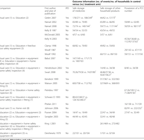
The example data comes from a recently updated Cochrane systematic review of home safety education and provision of safety equipment for injury prevention in children [31]. The models developed in this paper are applied to a subset of the review evidence relating to the prevention of poisoning injuries. Table 1 presents the data from 22 studies for the following outcomes:

a) Safe storage of medicines

b) Safe storage of other household products (e.g. cleaning products) and

Table 1 Summary of the available evidence

Outcome information (no. of events/no. of households in control versus (vs.) treatment arm)

Comparison First author

and year of publication

IPD Safe storage of medicines

Safe storage of other household products

Possession of a PCC number

Usual care (1)vs.Education (2) Gielen 2007 Yes 178/271 vs. 188/249Ɨ 44/62 vs. 57/73Ɨ

Nansel 2002 Yes 83/89 vs. 79/85 65/89 vs. 66/85 59/89 vs. 63/85

Nansel 2008 Yes 72/74 vs. 140/144† 59/73 vs. 117/144† 50/59 vs. 90/119† Kelly B 1987 No 54/54 vs. 55/55 43/54 vs. 49/55

McDonald 2005 No 4/57 vs. 6/60 3/57 vs. 6/61

Kelly N 2003 No 45.56/136.68 vs.

112.95/137.63*

Usual care (1)vs. Education + free/low cost safety equipment (3)

Clamp 1998 Yes 68/82 vs. 79/83 49/82 vs. 59/83

Woolf 1987 No 29/143 vs. 47/119

Woolf 1992 No 60/151 vs. 89/150 59/151 vs. 117/150

Usual care (1)vs.Education + equipment (3)vs. Education + equipment + home safety inspection (4)

Babul 2007 Yes 147/149 vs. 171/173 vs. 160/163

Usual care (1)vs.Education + equipment + home safety inspection (4)

Hendrickson 2002 Yes 14/40 vs. 34/38 8/40 vs. 34/38

Swart 2008 No 70.26/79.58 vs. 74.07/80* 46.86/57.96 vs. 50.87/58.27*

Kendrick 1999 Yes 317/367 vs. 322/363

Usual care (1)vs.Education + equipment + fitting (5)

Watson 2005 Yes 683/738 vs. 712/762 327/669 vs. 368/693

Usual care (1)vs.Education + home safety inspection (6)

Petridou 1997 No 67.26/100.12 vs.

71.08/97.83*

Usual care (1)vs.Education + equipment + home safety inspection + fitting (7)

Schwarz D 1993 No 88.42/248.37 vs. 128.16/248.37*

Phelan 2011 No 16/138 vs. 71/139

Usual care (1) vs.Home visit (8) Johnson 2006 No 82/91 vs. 222/232†

Education (2)vs.Education + equipment (3) Posner 2004 Yes 14/47 vs. 19/49 22/47 vs. 34/49 27/47 vs. 35/49

Education (2) vs. Education + equipment + fitting (5)

Sznajder 2003 Yes 44/49 vs. 43/45 32/41 vs. 40/48

Education + equipment + home safety inspection (4) vs. Education + equipment + home safety inspection + fitting (7)

King J 2001 No 261/469 vs. 273/482

Education + equipment (3) vs. Equipment (9)

Dershewitz 1979 No 22/101 vs. 20/104 1/101 vs. 0/104

Treatment abbreviation and codes:

Usual care = UC (1). Education = E (2).

Education + free/low cost equipment = E + FE (3).

Education + equipment + home safety inspection = E + FE + HSI (4). Education + equipment + fitting = E + FE + F (5).

Education + home safety inspection = E + HSI (6).

Education + equipment + home safety inspection + fitting = E + FE + HSI + F (7). Education + home visit = E + HV (8).

Free/low cost equipment = FE (9).

Thirteen of the 22 studies considered at least two of the three outcomes. Of these, 8 considered storage of medicines and storage of other household products, 2 considered storage of other household products and pos-session of a PCC telephone number, and 3 considered all three outcome measures. Individual patient data (IPD) were available for 8 of the 13 studies, of which 7 were in a format suitable for the analysis reported here as explained by the footnotes in Table 1.

We classified the interventions trialled in the 22 stud-ies into 9 relatively homogenous treatment packages:

1) Usual care (UC) 2) Education (E)

3) Education + provision of free/low cost equipment (E + FE)

4) Education + provision of free/low cost equipment + home safety inspection (E + FE + HSI)

5) Education + provision of free/low cost equipment + fitting of equipment (E + FE + F)

6) Education + home safety inspection (E + HSI)

7) Education + provision of free/low cost equipment + home safety inspection + fitting of equipment (E + FE + HSI + F)

8) Education + home visit (E + HV)

9) Provision of free/low cost equipment (FE).

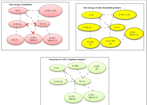
Figure 1 shows the comparisons between the inter-ventions that were made by individual studies and the number of comparisons in each network. All studies compared 2 intervention strategies, except Babul et al. (2007) [33] which compared 3 strategies. Data on each outcome was not available for all interventions; i.e. for the storage of medicines and other household products outcomes, interventions E + HSI and E + HV were not investigated in any of the included studies, and for possession of a PCC number interventions, E + FE + F and FE were not available.

Methods

In this section, we first present the NMA statistical model for one binary outcome measure and then extend it to

Safe storage of medicines

E+FE+ F (5)

UC (1)

E+FE+ HSI+F (7) E+FE (3)

E+FE+ HSI (4) E (2)

1 5 1

1 2

1 2

1

FE (9) 1

Safe storage of other household products

E+FE+ F (5)

UC (1)

E+FE+ HSI+F (7) E+FE (3)

E+E+ HSI (4) E (2)

1 ₅ 1

2

3 1

FE only (9)

1

1

Possession of a PCC telephone number*

UC (1)

E+HV (8)

E+FE (3)

E+FE+ HSI (4)

E+FE + HSI+F (7) E (2)

1 3 1

1 1

E+HSI

1

2

compare multiple interventions across multiple outcomes. Throughout the paper, we refer to these single and multiple outcome models as univariate and multivariate NMAs re-spectively. Where studies report multiple outcomes, these will not be independent as each household provides infor-mation on the different outcome measures within interven-tion arms. The multivariate model takes this correlainterven-tion structure into account by allowing the intervention effects measured by one outcome to be correlated with the inter-vention effects measured by other outcomes.

Model 1: Univariate NMA

Given arm-level binary data of the form presented in Table 1, a random effects NMA may be specified using the method of Lu and Ades [20]. It is assumed that the occurrence ofrikevents out of a total ofnikhouseholds in thekth-arm (k = A,B,C,….,) of theith-study follow a bino-mial distribution with underlying event probabilitypik:

rik_eBinomialðpik; nikÞ; logitð Þ ¼pik θik θik¼ _μμib

ibþδi bkð Þ

if k¼b if _k> _b

b¼A;B;C;

ð1Þ

δi bkð Þ_eNormal dð Þbk ¼dð ÞAk−dð ÞAb ; σ2ð Þbk

Note: dAA¼0

ð2Þ

whereμibis a study-specific baseline effect (i.e. the log-odds for the control group in studyiwith baseline treatment b),δi(bk)is a study-specific log-odds ratio,d(bk)is the pooled effect of treatment k relative to treatment b (a quantity usually of interest in a meta-analysis) and σ2

bk

ð Þ is the

between-study variance or heterogeneity parameter. Ran-dom effects NMA assumes that intervention effects are exchangeable across the network regardless of whether or not treatments b andk are included in studyi[18]. This assumption implies that the pooled effects d(bk), can be expressed as functions of basic parameters with reference to a common comparator or baseline treatment (i.e.d(bk)= d(Ak)−d(Ab)) [24]. Throughout this paper, we take usual care (UC) intervention to be the reference or ‘baseline’ treatment (i.e. UC is taken as treatmentAof equation (2) above). Multi-arm studies (i.e. studies with more than 2 treatment groups) present a special problem in network meta-analysis because they produce evidence on multiple treatment effects that are correlated through sharing a common reference or‘baseline’treatment. Under a homo-genous variance assumption (σ2

bk

ð Þ¼σ2), the covariance

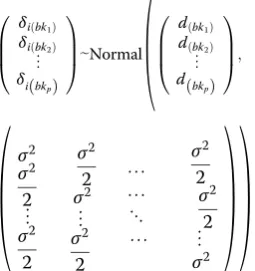
between any two effects that share a common reference treatment is σ₂2 [20]. The homogeneous variance assump-tion allows for the distribuassump-tion of effects (in a study with an arbitrary number of arms) to be expressed as a uni-variate marginal distribution and a series of uniuni-variate conditional distributions. Specifically, for the ith-study

with p + 1 arms and p treatment effect estimates

relative to the reference treatment, if

δi bkð 1Þ

δi bkð 2Þ

⋮

δ_{i bkð Þp}

0 B B @

1 C C AeNormal

dðbk1Þ dðbk2Þ

⋮ d_{ð Þbkp}

0 B B @

1 C C A;

σ2

σ2

2 ⋮ σ2

2 σ2

2 σ2

⋮ σ2

2 ⋯ ⋯ ⋱ ⋯

σ2

2 σ2

2 ⋮ σ2

!!

ð3Þ

then the marginal and conditional univariate distribu-tions for armj, given the previous 1,⋯, (j−1) arms are:

δi bkð 1ÞeNormal dðbk1Þ; σ 2

for j¼1:

δ_{i bkð Þjj} δi bkð 1Þ

⋮

δ_{i bkð j−1Þ}

0 @

1

AeNormal d_{ð Þþbkj} 1 j

Xj−1

t¼1

δi bkð tÞ−dðbktÞ

;ðjþ1Þ 2j σ

2

!

for j¼2;…;p

ð4Þ

The analysis is conducted within a Bayesian framework requiring prior distributions to be specified for all model parameters. Accordingly, we specified minimally inform-ative prior distributions corresponding to a Normal (0,103) prior distribution for the pooled mean effects relative to usual care,d(Ak)and the study-specific baseline effects,μib and a Uniform (0,2) prior distribution for the between-study standard deviation on the log odds ratio scaleσ[34].

Model 2: Multivariate NMA

We extend the univariate NMA model defined above to the multiple outcomes settings in order to account for correlations between intervention effects on dif-ferent outcomes. The method presented here follows

from Ades et al. (2010) NMA with competing risks

model [13] where only the within-study correlations are taken into account. We extend their method to account for the between-study correlation as well.

across outcomes. Instead, we use a Normal distribution on the log-odds scale to take account of the within-study cor-relations between outcomes. We assume that in each study iand for eachk-th arm, the estimatesθ^ikm of the observed

log-odds of an event on themth outcome (m= 1, 2,⋯,M) jointly follow a multivariate normal distribution:

^

θik1

⋮

^

θikM

0 @

1

AeNormal θik1

⋮ θikM

!

;

Sik ¼ s2

ik1 ⋯ r1ikMsik1sikM

⋱ ⋮

s2ikM

0 @

1 A

!

θik1

⋮ θikM

!

(

⋮ μibM

!

μ_ib1þδi bkð Þ1

⋮ μibMþδi bkð ÞM

0 @

1 A

if k¼b if k> b

for b¼A;B;C; …

ð5Þ

where (μib1, μib2,⋯, μibM) and (δi(bk)1, δi(bk)2,⋯, δi(bk)M) represent vectors of ‘true’ baseline and study-specific effects in study i with baseline treatment b respectively. The quantities θ^ik1; ^θik2;⋯; θikM

and (θik1, θik2,⋯, θikM) represent vectors of observed and ‘true’log-odds of re-sponse in arm k of study i and Sik is the associated within-study covariance matrix usually assumed known but estimated in practice from the data [35]. We calcu-lated ^θik1; ^θik2;⋯;θ^ikM

and the diagonal elements ofSik using standard formulae for log-odds and variance of the log-odds [2]. We applied a continuity correction by adding 0.5 to the numerators and 1 to the denominators of stud-ies with 0% or 100% event rate in one of the treatment arms [36,37]. The off-diagonals ofSikwere calculated from estimates of within-study correlations rmn

ik between

out-comesmandn(m≠n) in armkof studyiobtained from studies with IPD (see Additional file 1: Table S1). The method used to estimate the correlations from the IPD is described in the implementation section below.

When summarising evidence across multiple end-points, it is common to encounter instances where some studies do not report information for all outcomes of interest leading to incomplete vectors with missing study-specific effects for the outcomes not reported [5,10]. Such studies can be included in our model under the assumption that the effects for outcomes not re-ported are missing at random. When implemented using the WinBUGS software, the missing study effects and standard errors are coded as NA in the data, a strategy previously outlined in Bujkiewicz et al. [10] and Dakin et al. [28]. This enables WinBUGS to automatically

‘impute’ values for the missing information under miss-ing at random assumption with predicted distributions.

We refer to equation (5) as the within-study model and the model describing the distribution of the ‘true’ effects across studies (presented below) as the between-study model following standard terminology in multivariate meta-analysis [5,6,10,11,38,39]. For the network of two-arm trials, the between-study model for theith study is thus given by:

δi bkð Þ1 ⋮

δi bkð ÞM

0 @

1 AeNormal

dð Þbk1¼dð ÞAk1−dð ÞAb1 ⋮

dð ÞbkM¼dð ÞAkM−dð ÞAbM

0 @

1

A_{; Σð Þbk}

0 @

1 A

Σð Þbk ¼ σ2

bk

ð Þ1 ⋯ ρ1bkMσð Þbk1σð ÞbkM

⋱ ⋮

σ2

bk

ð ÞM

0 @

1 A

ð6Þ

where the ‘true’ effects δi(bk)m (m= 1, 2,⋯,M) jointly follow a Normal distribution with mean effects d(bk)m. The parameters in equation (6) have the same inter-pretation as in equation (2) except that they are now specific to each outcome. The covariance matrix Σ(bk) contains terms for the between-study variances, σ2

bk ð Þm

for each outcome m and the between-study correla-tionsρmn

bk between effects measured by outcomemand n (_m≠_n) specific to each _k versus _b comparison. Fit-ting the full model would thus require a large number of possibly multi-arm studies in order to make Σ(bk) identifiable [5,13]. The number of parameters in Σ(bk), can however be reduced if reasonable assumptions can be made about the covariance structure. In particular, most practical applications of NMA methods involve the assumption of a common between-study variance across treatment arms, often referred to as a homogenous vari-ance assumption [18,40,41]. Therefore, to simplify Σ(bk) we make the additional assumption in this context of a common between-study correlation (ρmn

bk ¼ ρmn)

lead-ing to the followlead-ing simplified between-study covari-ance structure for two-arm studies:

δi bkð Þ1

⋮

δi bkð ÞM

0 @

1 AeNormal

dð Þbk1¼dð ÞAk1−dð ÞAb1

⋮

dð ÞbkM¼dð ÞAkM−dð ÞAbM

0 @

1 A_;ΣðMMÞ 0

@

1 A

ΣðMMÞ¼ σ2

1 ⋯ ρ1M σ1σM

⋱ ⋮

σ2

M

0 @

1 A

ð7Þ

where, as in the univariate case, σm represent the com-mon between-study standard deviation or heterogeneity parameter specific to outcomem.

To include multi-arm studies in our model, we extend equations (3) and (4) to the multiple outcome setting. We show in Appendix A, that under evidence consistency and the homogenous between-study covariance structure (σ2

bk

to the multiple outcome settings by formulating the distribu-tion of effects in a multi-arm studyiwithp + 1arms report-ing onm= 1, 2,⋯,Moutcomes as follows:

wherepis the number of treatment effect estimates.The corresponding marginal and conditional distributions for armj, given the previous 1,⋯, (j−1) arms are:

δi bkð 1Þ1

⋮

δi bkð 1ÞM

0 @

1 AeNormal

dðbk1Þ1

⋮ dðbk1ÞM

0 @ 1 A_; 0 @

ΣðMMÞ¼ σ2

1 ⋯ ρ1M σ1σM

⋮ ⋱ ⋮

ρM1 _σ

1σM ⋯ σ2M

0 @

1 A

! forj¼1

δi bkð Þj1 ⋮ δi bkð ÞjM

0 B @ 1 C A

δi bkð 1Þ1 ⋮ δi bkð 1ÞM 0 @

1 A

δi bkð 2Þ1 ⋮ δi bkð 2ÞM 0 @

1 A

⋮ δi bkð j−1Þ1

⋮ δi bkð j−1ÞM 0 B @ 1 C A 0 B B B B B B B B B B B B B B B B B B B @ 1 C C C C C C C C C C C C C C C C C C C A eNormal

dð Þbkj1þ

1 j

Xj−1

t¼1

δi bkð tÞ1−dðbktÞ1

⋮

dð ÞbkjMþ

1 j

Xj−1

t¼1

δi bkð tÞM−dðbktÞM

0 B B B B B @ 1 C C C C C A;Σ

0

¼ðjþ1Þ

2j ΣðMMÞ 0 B B B B B @ 1 C C C C C A

forj¼2;…;p

ð9Þ

To complete model 2, μibmand d(1k)mare given min-imally informative prior distributions:

μibm; dð Þ1kmeNormal 0; 103

Prior distributions also need to be specified for Σ(M×

M) which, in general, is non-trivial because of the posi-tive definite constraint. Initially we specified an Inverse-Wishart distribution [42]:

ΣðMMÞeInverse−WishartðK;MÞ

whereKis M×Mscale matrix and Mis the total num-ber of outcomes. Specifying minimally informative Inverse-Wishart prior distribution is, however, problem-atic, especially when the amount of data is small relative to the dimensions of Σ(M×M) as is the case for our example data. Therefore, to allow for flexibility in for-mulating a prior distribution for Σ(M×M), we also followed a strategy outlined by Lu and Ades (2009) [43] and more recently by Wei and Higgins (2013) [39] to express Σ(M×M) in terms of a diagonal matrix of standard deviations V1/2and squared positive semi-definite matrix of correlations R based on a separation strategy (Barnardet al.[44]):

ΣðMMÞ¼ V1=2R V1=2 δi bkð 1Þ1

⋮

δi bkð 1ÞM

0 @

1 A

δi bkð 2Þ1

⋮

δi bkð 2ÞM

0 @

1 A

⋮

δi bkð Þp1

⋮

δ_{i bkð ÞpM}

0 B @ 1 C A 0 B B B B B B B B B B B B B B @ 1 C C C C C C C C C C C C C C A eNormal

dðbk1Þ1

⋮ dðbk1ÞM

0 @

1 A

dðbk2Þ1

⋮ dðbk2ÞM

0 @

1 A

⋮ dð Þbkp 1

⋮ d_{ð ÞbkpM}

0 B @ 1 C A 0 B B B B B B B B B B B B B B @ 1 C C C C C C C C C C C C C C A

; ΣðMpMpÞ

0 B B B B B B B B B B B B B B @ 1 C C C C C C C C C C C C C C A

ΣðMpMpÞ¼

σ2

1 ⋯ ρ1Mσ1σM

⋮ ⋱ ⋮

ρ1M_σ

1σM ⋯ σ2M

0 @ 1 A 1 2 σ2

1 ⋯ ρ1Mσ1σM

⋮ ⋱ ⋮

ρ1M_σ

1σM ⋯ σ2M

0 @

1 A ⋯ 1

2

σ2

1 ⋯ ρ

1M_σ

1σM

⋮ ⋱ ⋮

ρ1M_σ

1σM ⋯ σ2M

0 @

1 A

σ2

1 ⋯ ρ1Mσ1σM

⋮ ⋱ ⋮

ρ1M_σ

1σM ⋯ σ2M

0 @

1 A _⋮ 1

2

σ2

1 ⋯ ρ1Mσ1σM

⋮ ⋱ ⋮

ρ1M_σ

1σM ⋯ σ2M

0 @ 1 A ⋱ ⋮ σ2

1 ⋯ ρ1Mσ1σM

⋮ ⋱ ⋮

ρ1M_σ

1σM ⋯ σ2M

0 @ 1 A 0 B B B B B B B B B B B B B B B B B @ 1 C C C C C C C C C C C C C C C C C A 0 B B B B B B B B B B B B B B B B B @ 1 C C C C C C C C C C C C C C C C C A

where the off-diagonal elements ofRcontain correlation terms and diagonal elements equal 1. Lu and Ades [43] and also Wei and Higgins [39] showed that R can be written asR = LTLusing Cholesky decomposition where

L is an upper triangular matrix. The spherical para-meterization technique [39,43] can be used to expressR in terms of sine and cosine functions of the elements in

L. Using this later technique, we specified Uniform (0,π) prior distributions for the spherical coordinate φmn in our model to ensure that elements of the correlation matrix R lie in the interval (−1,1). Finally, the elements of V1/2 correspond to the between-study standard de-viation terms in Σ(M×M) and are given independent Uniform (0,2) prior distributions as in the univariate case (model 1).

Model 3: Borrowing strength across interventions and outcomes

From Table 1, it can be seen that none of the studies had considered the interventions E + HSI and E + HV for storage of medicines and storage of other household products. Similarly, interventions E + FE + F and FE were not trialled by any of the included studies on possession of a PCC number. To estimate the full set of 24 basic intervention effects relative to usual care from 9 inter-ventions on 3 outcomes, we applied methods originally proposed by DuMouchel and Harris [29] and revisited by DuMouchel and Groer [45] and Jones et al.[30]. We assume that the pooled effects of treatmentkrelative to usual care intervention d(Ak)m, can be expressed as a sum of treatment-specific effectαkand outcome-specific effectγm. This assumption replaces the minimally inform-ative prior distribution N(0, 103) specified for d(Ak)m in model 2 with:

dð ÞAkmeNormal αkþγm; τ2

k¼2; 3; ⋯K; m¼1;2; M

ð10Þ

where Kis the total number of treatments being evalu-ated across M outcomes, and for k= 1 (i.e. reference treatment A), d(Ak)m equal to zero. Note that on the logarithmic scale, this would imply that the ratio of any intervention effects is constant across outcomes as the γmcancel, i.e.

dð Þbkm¼ dð ÞAkm−dð ÞAbm

eNormal αk−αb;2τ2

ð11Þ

Equation (10) thus embodies an assumption of equal or constant relative potency of treatments across out-comes which imply exchangeability of the relative effects between the non-reference/baseline treatments indicated by equation (11). For our example dataset, this implies that missing intervention effects for comparisons with the usual care intervention can be predicted directly

from equation (10) as a linear combination ofγmand αk assuming that each treatment effect relative to usual care is reported on at least one outcome. The missing intervention effects between non- reference/baseline treatments if required can similarly be predicted directly from the model as linear combinations of the interven-tion effects relative to usual care.

The parameter τ controls the accuracy of the constant relative potency assumption. Values ofτclose to zero would thus indicate a high degree of confidence (and support from the data) in the parallelism of effect profiles across outcomes and the constant relative potency assumption. Conversely, larger values ofτwould indicate otherwise.

Multi-arm studies are included in model 3 based on equations (8) and (9) in the same way as in model 2. To

complete model 3, the parameters αk, γm and τ are

given minimally informative prior distributions. For the mean effects, this is a normal distribution with zero mean and large variance:

αk; γmeNormal 0; 103

We give τa Uniform (0, 2) prior distribution, consid-ered to be minimally informative on the log-odds ratio scale. Sensitivity analyses were conducted to assess the impact of specifying alternative prior distributions for τ that are also considered minimally informative [46]:

i. Normal prior distribution centred on 0 with large variance and constrained to be positive,τ~ N (0, 102),τ≥0

ii. Gamma prior distribution placed on the precision: τ−2

~ Gamma(0.001, 0.001).

The results of the sensitivity analyses are presented in Additional file 1: Figure S1.

There is a limitation to the number of data (i.e. inter-vention effects relative to the usual care) on outcomes allowed to be missing for the model hyper-parameters to be identifiable. ForKinterventions andMoutcomes, there will be (K−1) ×Mequation (10) that are used to estimate a total of (K−1) +M hyper-parameters (i.e. (K−1) ofαk andM ofγmhyper-parameters). Therefore no more than ((K−1) ×M)−((K−1) +M) missing values in total are allowed. For example, forK= 3 treatments and M = 2 out-comes, data has to be available on both outcomes for both treatment comparisons with the baseline when the prior dis-tributions are non-informative. When large number of data on outcomes is missing, placing informative prior distribu-tions on the hyper-parameters can improve convergence.

Implementation of the models

we specified an inverse-Wishart prior distribution for the between-study covariance matrix Σ(M×M) whilst in model 2b, we specified a prior distribution for Σ(M×M) based on the separation strategy. All four models allowed for multi-arm trials to be included in the ana-lysis. To fit the multivariate NMA models, the quan-tities ðθ^ik1; θ^ik2; θ^ik3Þ and the diagonals of Sik were

estimated using standard 2×2–table formulae [2].

Next, we obtained estimates of the within-study corre-lations from the IPD studies using the following three methods: i) Pearson correlation coefficient between the observed outcome events ii) Bootstrapping as described in Daniel and Hughes (1998), and iii) Generalised Estimating Equations (See details in Additional file 1). All three methods produced identical estimates of the correlations between pairs of outcome specific log-odds of event from each IPD study (Additional file 1: Table S1). Therefore, we formulated informative prior distributions for the correl-ation terms in Sik of equation (5) using the estimates of the correlations between the observed outcome events (Pearson correlation) as follows:

rmn

ik eUniformðamn;bmnÞ with

amn_¼rmn−

ffiffiffiffiffiffiffiffiffiffiffiffiffiffiffiffiffiffiffiffiffiffiffiffiffiffiffiffi 12var rð mnÞ

p

2

! and

bmn¼rmn_þ

ffiffiffiffiffiffiffiffiffiffiffiffiffiffiffiffiffiffiffiffiffiffiffiffiffiffiffiffi 12var r_ð mn_Þ

p

2

!

where rmnik is the within-study correlation between the

outcomes m and n effects measured on the log-odds scale in arm k of studyi, and rmn _{and var (r}mn_{)are the} mean and variance of the within-study correlation be-tween outcomes m and n effects measured by IPD respectively.

We also assessed consistency of the evidence within each network using a method based on node splitting [24]. We found no evidence of conflict between the dir-ect and indirdir-ect sources (Additional file 1: Table S2) in all three outcome networks.

We fitted all models described above in WinBUGS [47] using Markov Chain Monte Carlo (MCMC) simula-tions. The univariate models were fitted separately for each outcome using WinBUGS code available from Dias et al. [48]. The WinBUGS code for the multivariate models is provided in the appendices 1 and 2 of the Additional file 1. Convergence was assessed by examin-ation of the trace and autocorrelexamin-ation plots and the Rubin-Gelman statistic after running 400 000 simula-tions and discarding the first 200 000 samples as ‘burn in samples’.

Results

Univariate and multivariate analyses

Parameters of interest were the posterior median esti-mate (and 95% credible intervals) of the pooled inter-vention effects relative to the usual care interinter-vention and the posterior median estimate (and 95% credible in-tervals) of the between-study standard deviation and correlation terms. Summary forest plots displaying ef-fectiveness estimates relative to usual care on the odds ratio (OR) scale are presented in Figure 2. It can be seen that, all 4 models produced broadly similar estimates when the treatment effect is not extreme compared to the other effect estimates for the same outcome. Com-pared to the univariate analysis, the multivariate models produced noticeably less extreme estimates of interven-tion effects. This can be seen in the effect of FE + HSI (3) on possession of PCC number being shifted towards the line of no effect from an OR of 39.35 (95% CrI 2.37 to 732.30) in model 1 to 23.55 (95% CrI 1.39, to 456.80) in model 2a, 20.37 (95% CrI 0.72, to 706.00) in model 2b and 4.20 (95% CrI 1.59 to 13.16) in model 3. Similarly, the OR for FE (9) on safe storage of other household products shifted from 0.37 (95% CrI 0.00 to 15.10) in model 1 to 1.81 (95% CrI 0.63, to 5.37) in model 3.

Posterior median and 95% credible intervals of the between-study standard deviations and correlations are presented in Table 2. The posterior medians of the between-study correlations from the multivariate models were small and estimated with considerable uncertainty (i.e. all had large variances). Estimates of the between-study standard deviations were broadly similar for the univariate NMA (model 1) and the multivariate NMA using the separation strategy (model 2b), and relatively high for multivariate NMA using the inverse-Wishart prior distribution (model 2a).

Borrowing strength across outcomes

Figure 2Summary forest plot of intervention effects relative to usual.Outcomes are safe storage of medicines, safe storage of other household products and possession of a PCC telephone number. Model 1: Univariate NMA. Model 2a: Multivariate NMA (Wishart prior

distribution). Model 2b: Multivariate NMA (separation strategy). Model 3: Multivariate NMA allowing for the relative effects between non-usual care interventions to be exchangeable across outcomes. Effect estimate for which direct study data was not available are indicated by xx on the forest plot. Intervention components: E = Education, FE = low cost/free equipment, HSI = Home safety inspection, HV = Home visit and F= Fitting of equipment.

Table 2 Posterior median and 95% credible intervals of the between-study standard deviation and correlation parameters

Parameter Description/prior distribution Model 1: univariate

Model 2a: Multivariate using inverse-Wishart prior distribution for Σ(M×M)

Model 2b: Multivariate using a separation strategy to specify priors for elements ofΣ(M×M)

Model 3: Multivariate with extrapolation of effects across outcomes

σ1 Between-study standard deviation:

safe storage of medicines

0.26 (0.03, 1.02) 0.58 (0.33, 1.18) 0.27 (0.01, 1.08) 0.23 (0.01, 0.80)

σ2 Between-study standard deviation:

safe storage of other household products

0.56 (0.13, 1.27) 0.62 (0.35, 1.15) 0.47 (0.04, 1.18) 0.31 (0.01, 0.81)

σ3 Between-study standard deviation:

PCC

1.16 (0.57, 1.93) 0.94 (0.53, 1.99) 1.18 (0.57, 1.93) 1.08 (0.58, 1.85)

τ Primary analysis:_τ~Uniform(0, 2) - - - 0.10 (0.01, 0.53)

τ Sensitivity analysis:_τ~ Normal (0, 102_),

τ≥0

- - - 0.11 (0.00, 0.56)

τ Sensitivity analysis:τ2~ Inverse− Gamma (0.001, 0.001)

- - - 0.08 (0.02, 0.36)

ρ12 _{Between-study correlation [medicines,}

other household products]

- 0.03 (₋0.73, 0.76) 0.05 (₋1.00, 1.00) 0.45 (₋0.99, 1.00)

ρ13

Between-study correlation [medicines, PCC]

- 0.06 (−0.80, 0.81) 0.20 (−1.00, 1.00) 0.50 (−0.98, 1.00)

ρ23 _{Between-study correlation [Other}

household products, PCC]

The posterior median and 95% credible intervals of intervention effects relative to usual care were un-affected by placing alternative minimally informative prior distributions on τ (Additional file 1: Appendix 2).

The posterior median and credible intervals for τ

(Table 2) were similarly not sensitive to the choice of prior distribution placed onτin the primary and sensi-tivity analyses. The posterior median estimates ofτwere all close to zero, which suggest that assumptions about the parallelism of effect profiles across outcomes is sup-ported by the data. The estimates of τwould thus sug-gest with 95% probability, that based on the information in our example dataset, the extrapolation model could be accurate to within a factor of about e(2 × 0.10)= 1.24 (95% CrI 1.01 to 2.87).

Discussion

We have presented methods for simultaneous compari-son of multiple treatments across multiple outcome measures while preserving the internal randomisation of individual studies. Our method may be viewed as an ex-tension of Ades et al.’s (2010) NMA with competing risks paper [13] wherein only the within-study correl-ation is taken into account. We have extended their method to account for the dependency between out-come effects across studies as well as within-studies.

In this particular application of the multivariate ap-proach, accounting for the correlation between out-comes alone (models 2a and 2b) did not reduce the uncertainty around estimates of intervention effects compared to analysing each outcome separately (model 1). Assuming that intervention effects are exchangeable across outcome did however lead to a modest re-duction in uncertainty around effectiveness estimates (model 3).

The between-study correlations were estimated with considerable uncertainty (Table 2) and appear to have little impact on overall effect estimates. This may be because the between-study correlation arises due to, among other things, differences in study-level charac-teristics that also give rise to between-study heterogen-eity in a meta-analysis. Based on a criterion outlined in Spiegelhalteret al. [49] the posterior median estimates of the between-study standard deviations,σ1andσ2on the log odds ratio scale (Table 2) could be interpreted as indicating evidence of low to moderate heterogeneity for storage of medicines and storage of other household products outcomes. Only the estimates for possession of poison control centre number exhibited a consider-able degree of heterogeneity. Consequently, the posterior medians of the between-study correlations were small. There was therefore very little gain (in terms of increasing the precision of estimates) from formulating the between-study covariance structure described for the analysis

presented here. Accounting for the between-study correl-ation is likely to be beneficial in situcorrel-ations where the between-study variance (heterogeneity) is large relative to within-study variances.

We opted to incorporate the within-study correlation through the arm-specific effects (log-odds) rather than the study-specific treatment difference (log-odds ratio) as is often done in multivariate meta-analysis [3,4,15,38]. This approach greatly simplifies the likelihood for multi-arm studies because treatment multi-arms can be considered independent as a consequence of randomisation. Hence, there is no requirement to account for the additional correlations between effect estimates which share a com-mon comparator treatment in the model likelihood [50]. The arm-based approach is also likely to be useful when (as is typical with many practical application of multi-variate meta-analysis) the within-study correlations are not available [10,12,15,51] and have to be obtained from an external source such as expert opinion [14]. In such situations, formulating questions about corre-lations between outcome-specific event probabilities (which can be used directly in an arm-based approach) is more likely to be intuitive and easily understood by

non-statistician healthcare experts than questions

about correlations between intervention effects. It is acknowledged however, that the correlations between the intervention effects if required can easily be ob-tained from the correlations between the outcomes [14,51].

At the between-study level, we assumed a common correlation structure across treatments in addition to the common variance assumption underlying most practical application of NMA methods. The common correlation assumption implies that if several separate multivariate meta-analyses were conducted with the same outcomes, each with a different set of k versus b comparison, the assumption is that the between-study correlations would be the same across the different sets of bkcomparisons. We suggested this structure to simplify the covariance structure and reduce the number of parameters in the model. Appropriateness of such modelling assumptions would need to be considered carefully and assessed when it is feasible to do so.

Gamma prior distribution (which is the univariate analogue of the Inverse-Wishart prior distribution) can lead to an overestimation of the heterogeneity parameter when the true value is close to 0 [46,52]. As an alternative to an inverse-Wishart prior distribution therefore, we followed the spherical decomposition technique suggested by Lu and Ades [43]. This parameterization offered greater flexibility in formulating independent prior distribu-tions for the standard deviation and correlation terms in Σ(M×M).

An obvious limitation to implementation of the multi-variate models presented in this paper is the limited availability of data including i) the problem of missing within-study correlations and ii) the requirement for a relatively large number of studies to estimate all model parameters. The problem of missing within-study corre-lations has traditionally hampered the widespread appli-cation of multivariate meta-analysis [7,10,15]. In our example, IPD was available from a proportion of the in-cluded studies and we have used correlations estimated from the IPD to formulate informative prior distribu-tions for the within-study model. Alternative approaches to dealing with missing within-study correlations when IPD is not available include: i) using the observed correl-ation from the summary study-specific effects [12], ii) eliciting information about the correlations from exter-nal sources such as clinical experts [14] and iii) specify-ing ‘vague’ prior distributions for analysis conducted within a Bayesian framework [6].

The second data issue concerns the number of stud-ies needed to estimate the full unstructured between-study covariance matrix presented in equation (6). We anticipate a large number of multi-arm studies report-ing across the three outcomes will be needed to iden-tify Σ(bk) and estimate all model parameters. This can be problematic considering the fact that most applica-tions of network meta-analysis typically include mostly two-arm studies with very small numbers of multi-arm studies. Even with the simplification of the between-study covariance matrix given in equation (5), a rela-tively large number of studies in comparison to the total number of outcomes being considered may still be needed. We are unable to answer the question of how many studies should be considered large enough for a NMA with multiple outcomes. As a guide, Wei and Higgins [39] recently estimated 15, 27 and 42 studies as a minimum for multivariate pairwise meta-analysis with two, three and four-outcomes respect-ively. Hence, we believe an even larger number of studies will be required for the NMA with multiple outcomes.

Another limitation of the multivariate models presented here is that they rely on the normal approximation to binomial distribution to incorporate the within-study

correlations in the model. The normal approximation frequently fails and may not provide adequate fit to the data in the presence of studies with zero or a small number of events, necessitating use of continuity cor-rections. We were unable to use the exact binomial distribution as our primary interest was to develop models for summary binary data where outcomes are not mutually exclusive, and where it is not reasonable to assume that within-study correlations are zero so that the likelihood factorises easily as in Arends et al. [3]. Further methodological investigations into model-ling multivariate summary data that is not normally distributed will therefore be useful. An example is pro-vided in Chu et al. [53] where parameterization of the within-study model enabled the special case of diag-nostic sensitivity and specificity to be jointly modelled with disease prevalence using a trivariate binomial likelihood. In the interim, an alternative formulation which bypasses the need for approximating normal distributions is to directly model the IPD where this is available. This will require extending Saramagoet al.’s [54] NMA model with aggregate and individual partici-pant level data from single outcome to multiple outcome settings.

We assessed the consistency of each outcome network separately using the method of node splitting [24]. We found no evidence of conflict between the direct and in-direct sources on pairwise contrasts that have both sources of evidence in model 1. We did not assess the consistency of the multivariate estimates partly because we are unaware of current methods for carrying out this type of assessment. We are investigating extensions of the node-split method to multiple outcome networks and investigate the effect of jointly synthesising evidence across multiple endpoints on evidence consistency in a simulation study.

Our initial motivation for a multiple outcome NMA was to estimate intervention effects for all the outcomes, including effects of interventions on outcomes not con-sidered by any of the studies included in the analysis. This requires the correlation structure between effects on multiple outcomes to be appropriately modelled and

also ensuring the mechanism of “borrow strength”

being measured on different scales (e.g. where one out-come reports a weighted mean difference and another outcome reports a log-odds ratio) as such estimates will differ in terms of the precision with which they are estimated.

Conclusion

Our aim in this paper was to present methods for simul-taneous comparison of multiple treatments across multiple outcome measures while preserving the in-ternal randomisation of individual studies. Application of the method to the poison prevention data yielded similar point estimates of treatment effect to those obtained from a univariate NMA but the uncertainty around the multivariate estimates increased or de-creased depending on the prior distribution specified for the between-study covariance structure. The proposed method followed the usual hierarchical approach to multivariate meta-analysis where correlations between outcomes are modelled at the within-study and or be-tween-study levels.

Appendix A

Between-study covariance for multi-arm studies reporting multiple outcomes

For a multi-arm study iwithKtreatments labelledA, B, C,…, Kreporting a total ofMoutcomes labelled1, 2,…, M. A random effects between-study model can be repre-sented as:

δi ABð Þ1 ⋮ δi ABð ÞM 0 @

1 A

δi ACð Þ1 ⋮ δi ACð ÞM 0 @

1 A

⋮ δi AKð Þ1

⋮ δi AKð ÞM 0 @ 1 A 0 B B B B B B B B B B B B B B @ 1 C C C C C C C C C C C C C C A eNormal

di ABð Þ1 ⋮ di ABð ÞM 0 @

1 A

di ACð Þ1 ⋮ di ACð ÞM 0 @

1 A

⋮ di AKð Þ1

⋮ di AKð ÞM 0 @ 1 A 0 B B B B B B B B B B B B B B @ 1 C C C C C C C C C C C C C C A

;ΣFULL

0 B B B B B B B B B B B B B B @ 1 C C C C C C C C C C C C C C A

ðA1Þ

Whereδi(Ak)mandd(Ak)mare study-specific and mean ef-fect of treatment k relative A (reference treatment) on outcomemin studyirespectively andΣFULLis the full

(K-1) × (K-1) blocks ofM×Mwithin-treatment between-outcome covariance matrix. The parameters in ΣFULL

have the following interpretation: (σ2

Ak

ð Þm) indicate the variance of the effect of treatmentk(k= B,C,⋯,K) relative toAon outcomemacross studies.

ρmn

Ak;Ak

ð Þ indicate the correlation betweenδi(Ak)mandδi(Ak)n (i.e. the correlation between the effect of treatmentkrelative toAon outcomemand the effect of treatmentkrelative to Aon outcomen(m≠n)) specific to theAkcomparison.

ρmm

Ah;Ak

ð Þ indicate the correlation betweenδi(Ah)mand δi

(Ak)m(i.e. the correlation between the effect of treatment

hrelative toAon outcomemand the effect of treatment krelative toA(h≠k) on outcomembecause they share a common comparatorA).

The diagonal block matrices inΣ_FULLthus carry terms for the between-study variance (σ2

Ak

ð Þm) while the

off-diagonal blocks carry terms for the between-study co-variance. We make two assumptions to simplify and re-duce the number of parameters in ΣFULL. First, we

assume homogenous variances for intervention effects within outcomes [20]. This implies σ2_{ð ÞAkm}¼σ2_m and ρmm

Ah;Ak

ð Þ¼ 12 as in the single outcome network

meta-analysis case [20,34]. Second, we make the assumption of homogenous between-study correlations for the intervention effects from different outcomes. Under this assumption we can expressρmn

Ah;Ah

ð Þ andρmnðAk;AkÞ in

terms of a common correlation parameterρmn by not-ing that for any 3-treatment(A, h, k)configuration, the

covariance between outcome m and n effects across

studies can be expressed as a covariance between two sums under evidence consistency:

δi hkð Þm;δi hkð Þn

¼COV δi Akð Þm−δi Ahð Þm

; δi Akð Þn−δi Ahð Þn

¼COV δi Akð Þm;δi Akð Þn

−COV δi Akð Þm;δi Ahð Þn

−COV δi Ahð Þm;δi Akð Þn

þCOV δi Ahð Þm;δi Ahð Þn

¼ ρmn Ak;Ak

ð ÞþρmnðAh;AhÞ−2ρmnðAk;AhÞ

σmσn

ðA2Þ

ΣFULL¼ σ2

AB

ð Þ1 ⋯ ρ1MðAB;ABÞσð ÞAB1σð ÞABM

⋮ ⋱ ⋮

ρ1M AB;AB

ð Þσð ÞAB1σð ÞABM ⋯ σ2ð ÞABM 0 @ 1 A ρ 11 AB;AC

ð Þσð ÞAB1σðACÞ1 ⋯ ρð1MAB;ACÞσð ÞAB1σðACÞM

⋮ ⋱ ⋮

ρ1M AB;AC

ð Þσð ÞAB1σðACÞM ⋯ ρðMMAB;ACÞσð ÞABMσðACÞM 0

@

1 A⋯ ρ

11 AB;AK

ð Þσð ÞAB1σðAKÞ1 ⋯ ρð1MAB;AKÞσð ÞAB1σðAKÞM

⋮ ⋱ ⋮

ρ1M AB;AK

ð Þσð ÞAB1σðAK;AKÞM ⋯ ρðMMAB;AKÞσð ÞABMσðAKÞM 0 @ 1 A σ2 AC

ð Þ1 ⋯ ρ1MðAC;ACÞσðACÞ1σðACÞM

⋮ ⋱ ⋮

ρ1M AC;AC

ð ÞσðACÞ1σðACÞM ⋯ σ2ðACÞM 0

@

1

A⋮ ρ

11 AC;AK

ð ÞσðACÞ1σðAKÞ1 ⋯ ρð1MAC;AKÞσðACÞ1σðAKÞM

⋮ ⋱ ⋮

ρ1M AC;AK

ð ÞσðACÞ1σðACÞM ⋯ ρðMMAC;AKÞσðACÞMσðAKÞM 0 @ 1 A ⋱ ⋮ σ2 AK

ð Þ1 ⋯ ρ1MðAK;AKÞσðAKÞ1σðAKÞM

⋮ ⋱ ⋮

ρ1M AK;AK

ð ÞσðAKÞ1σðAKÞM ⋯ σ2ðAKÞM 0

@

The homogenous between-study correlation assumption impliesρmn_ðAh;AhÞ¼ ρmn_ðAk;AkÞ¼ρmn andρmn_ðAk;AhÞ¼ 1₂ρmn for

the inequality −1≤ ρmn Ak;Ak

ð ÞþρmnðAh;AhÞ−2ρmnðAk;AhÞ

≤1 to hold. Substituting these expressions into equation (A1), we see that the between-study correlation terms equal ρmn _{in the diagonal block of matrices and} 1

2ρmn in the

off-diagonal block of matrices of in ΣFULL leading to

the following simplificationfollowing simplification of the between-study covariance matrix:

Finally by relabeling the reference treatment Aas b, (δi(AB)1,⋯,δi(AK)m) as δi bkð 1Þ1; ⋯;δi bkð ÞjM

and (d(AB)1, ⋯,

d(AK)M) as dðbk1ÞM; ⋯;dð Þbkj M

, equation (A3) can be

rewritten as equation (A4).

δi ABð Þ1

⋮ δi ABð ÞM

0 @

1 A

δi ACð Þ1

⋮ δi ACð ÞM

0 @

1 A

⋮ δi AKð Þ1

⋮

δi AKð ÞM

0 @ 1 A 0 B B B B B B B B B B B B B B @ 1 C C C C C C C C C C C C C C A eNormal

dð ÞAB1

⋮

dð ÞABM

0 @

1 A

dðACÞ1

⋮

dðACÞM

0 @

1 A

⋮

dðAKÞ1

⋮

dðAKÞM

0 @

1 A

;ΣðMpMpÞ

0 B B B B B B B B B B B B B B @ 1 C C C C C C C C C C C C C C A

with ΣðMpMpÞ¼

σ2

1 ⋯ ρ1Mσ1σM

⋮ ⋱ ⋮

ρ1M_σ

1σM ⋯ σ2M

0 @ 1 A 1 2 σ2

1 ⋯ ρ1Mσ1σM

⋮ ⋱ ⋮

ρ1M_σ

1σM ⋯ σ2M

0 @

1 A _⋯ 1

2

σ2

1 ⋯ ρ1Mσ1σM

⋮ ⋱ ⋮

ρ1M_σ

1σM ⋯ σ2M

0 @

1 A

σ2

1 ⋯ ρ1Mσ1σM

⋮ ⋱ ⋮

ρ1M_σ

1σM ⋯ σ2M

0 @

1 A_⋮ 1

2

σ2

1 ⋯ ρ1Mσ1σM

⋮ ⋱ ⋮

ρ1M_σ

1σM ⋯ σ2M

0 @

1 A

σ2

1 ⋯ ρ1Mσ1σM

⋮ ⋱ ⋮

ρ1M_σ

1σM ⋯ σ2M

0 @ 1 A 0 B B B B B B B B B B B B B B B B B @ 1 C C C C C C C C C C C C C C C C C A

ðA3Þ

δi bkð 1Þ1 ⋮ δi bkð 1ÞM

0 @

1 A

δi bkð 2Þ1 ⋮ δi bkð 2ÞM

0 @

1 A

⋮ δ_{i bkð Þp} 1

⋮ δ_{i bkð Þp M} 0 B @ 1 C A 0 B B B B B B B B B B B B B B @ 1 C C C C C C C C C C C C C C A eNormal

dðbk1Þ1 ⋮ dðbk1ÞM

0 @

1 A

dðbk2Þ1 ⋮ dðbk2ÞM

0 @

1 A

⋮ d_{ð Þbkp} 1

⋮ d_{ð Þbkp M} 0 B @ 1 C A 0 B B B B B B B B B B B B B B @ 1 C C C C C C C C C C C C C C A

; ΣðMpMpÞ

0 B B B B B B B B B B B B B B @ 1 C C C C C C C C C C C C C C A

Additional file

Additional file 1:(WinBUGS Code for model 2): Network meta-analysis of multiple outcome measures accounting for borrowing of information across outcomes.

Abbreviations

CrI:Credible interval; IPD: Individual patient data; MCMC: Markov Chain Monte Carlo; NMA: Network meta-analysis; PCC: Poison centre control number.

Competing interests

The authors declare that they have no competing interests.

Author’s contribution

FAA drafted the initial manuscript, conducted the analysis and coordinated contributions from all authors in drafting the final manuscript. NJC designed the study and revised the manuscript to improve general readability. SB contributed to developing the statistical analysis and interpretation of the results. SJH contributed to preparing the data for analysis, drafting the network diagrams and revision of the initial and final drafts. DK provided the data for analysis, defined the outcomes and interventions and revision of the final drafts.DRJ participated in designing the study and revision of the final manuscript. AJS conceived the original idea and participated developing the statistical model. All authors read and approved the final manuscript.

Acknowledgements

FAAis funded by the National Institute for Health Research (NIHR) under its Programme Grants for Applied Research programme (Reference Number RP-PG- 0407_–10231) to pursue a PhD in Public Health Evaluation of Interventions.

SBis supported by the MRC Methodology Research Programme (grant number MR/L009854/1).

Author details

1_{Biostatistics Group, Department of Health Sciences, University of Leicester,}

University Road, Leicester LE1 7RH, UK.2Division of Primary Care Community Health Sciences, Faculty of Medicine & Health Sciences, University of Nottingham, Nottingham NG7 2RD, UK.

Received: 8 January 2014 Accepted: 2 July 2014 Published: 21 July 2014

References

1. Cooper NJ, Sutton AJ, Ades AE, Paisley S, Jones DR, W. G. O. U. o. E. i. E. D: Models, Use of evidence in economic decision models: Practical issues and methodological challenges.Health Economics2007,16(12):1277–1286. 2. Sutton A, Abrams K, Jones DR, Sheldon TA, Song F:Methods for Meta-analysis

in Medical Research.Chichester: Wiley; 2000.

3. Arends LR, Voko Z, Stijnen T:Combining multiple outcome measures in a meta-analysis: an application.Statistics in Medicine2003,22(8):1335–1353. 4. Berkey CS, Hoaglin DC, Antczak-Bouckoms A, Mosteller F, Colditz GA:

Meta-analysis of multiple outcomes by regression with random effects.

Statistics in Medicine1998,17(22):2537–2550.

5. Jackson D, Riley R, White IR:Multivariate meta-analysis: Potential and promise.Statistics in Medicine2011,30(20):2481–2498.

6. Nam IS, Mengersen K, Garthwaite P:Multivariate meta-analysis.Statistics in

Medicine2003,22(14):2309–2333.

7. Riley RD, Abrams KR, Sutton AJ, Lambert PC, Thompson JR:Bivariate random-effects meta-analysis and the estimation of between-study correlation.BMC Medical Research Methodology2007,7.

8. Riley RD, Thompson JR, Abrams KR:An alternative model for bivariate random-effects meta-analysis when the within-study correlations are unknown.Biostatistics2008,9(1):172–186.

9. Kendrick D, Coupland C, Mulvaney C, Simpson J, Smith SJ, Sutton A, Watson M, Woods A:Home safety education and provision of safety equipment for injury prevention.Cochrane Database Systematic reviews2007, 1:CD005014.

10. Bujkiewicz S, Thompson JR, Sutton AJ, Cooper NJ, Harrison MJ, Symmons DPM, Abrams KR:Multivariate meta-analysis of mixed outcomes: a Bayesian approach.Statistics in Medicine2013,32(22):3926–3943.

11. Riley RD, Abrams KR, Lambert PC, Sutton AJ, Thompson JR:An evaluation of bivariate random-effects meta-analysis for the joint synthesis of two correlated outcomes.Statistics in Medicine2007,26(1):78–97.

12. Kirkham JJ, Riley RD, Williamson PR:A multivariate meta-analysis approach for reducing the impact of outcome reporting bias in systematic reviews.

Statistics in Medicine2012,31(20):2179–2195.

13. Ades AE, Mavranezouli I, Dias S, Welton NJ, Whittington C, Kendall T: Network meta-analysis with competing risk outcomes.Value Health2010, 13(8):976–983.

14. Efthimiou O, Mavridis D, Cipriani A, Leucht S, Bagos P, Salanti G:An approach for modelling multiple correlated outcomes in a network of interventions using odds ratios.Statistics in Medicine2014,33(13):2275–2287.

15. Riley RD:Multivariate meta-analysis: the effect of ignoring within-study correlation.Journal of the Royal Statistical Society Stat Soc2009,172:789_–811. 16. Rodgers M, Sowden A, Petticrew M, Arai L, Roberts H, Britten N, Popay J:

Testing Methodological Guidance on the Conduct of Narrative Synthesis in Systematic Reviews.Evaluation2009,15(1):49–73.

17. Lumley T:Network meta-analysis for indirect treatment comparisons.

Statistics in Medicine2002,21(16):2313_–2324.

18. Caldwell DM, Ades AE, Higgins JP:Simultaneous comparison of multiple treatments: combining direct and indirect evidence.British Medical

Journal2005,331(7521):897_–900.

19. Caldwell DM, Welton NJ, Ades AE:Mixed treatment comparison analysis provides internally coherent treatment effect estimates based on overviews of reviews and can reveal inconsistency.Journal of Clinical Epidemiology2010, 63(8):875–882.

20. Lu G, Ades AE:Combination of direct and indirect evidence in mixed treatment comparisons.Statistics in Medicine2004,23(20):3105_–3124. 21. Salanti G, Ades AE, Ioannidis JP:Graphical methods and numerical

summaries for presenting results from multiple-treatment meta-analysis: an overview and tutorial.Journal of Clinical Epidemiology2010,64(2):163–171. 22. Salanti G, Higgins JP, Ades AE, Ioannidis JP:Evaluation of networks of

randomized trials.Statistical Methods in Medical Research2008,17(3):279–301. 23. Salanti G, Marinho V, Higgins JP:A case study of multiple-treatments

meta-analysis demonstrates that covariates should be considered.

Journal of Clinical Epidemiology2009,62(8):857_–864.

24. Dias S, Welton NJ, Caldwell DM, Ades AE:Checking consistency in mixed treatment comparison meta-analysis.Statistics in Medicine2010, 29(7_–8):932_–944.

25. Hong H, Carlin BP, Chu H, Shamliyan TA, Wang S, Kane RL:Methods Research Report: A Bayesian Missing Data Framework for Multiple Continuous Outcome

Mixed Treatment Comparisons; 2013. Avaialable online from http://www.ncbi.

nlm.nih.gov/books/NBK116689/pdf/TOC.pdf.

26. Lu G, Ades AE, Sutton AJ, Cooper NJ, Briggs AH, Caldwell DM:Meta-analysis of mixed treatment comparisons at multiple follow-up times.Statistics in Medicine

2007,26(20):3681–3699.

27. Welton NJ, Cooper NJ, Ades AE, Lu G, Sutton AJ:Mixed treatment comparison with multiple outcomes reported inconsistently across trials: evaluation of antivirals for treatment of influenza A and B.Statistics in Medicine2008, 27(27):5620–5639.

28. Dakin HA, Welton NJ, Ades AE, Collins S, Orme M, Kelly S:Mixed treatment comparison of repeated measurements of a continuous endpoint: an example using topical treatments for primary open-angle glaucoma and ocular hypertension.Statistics in Medicine2011,30(20):2511_–2535. 29. DuMouchel WH, Harris JE:Bayes Methods for Combining the Results of Cancer

Studies in Humans and Other Species.Journal of the American Statistical

Association1983,78(382):293_–308.

30. Jones DR, Peters JL, Rushton L, Sutton AJ, Abrams KR:Interspecies extrapolation in environmental exposure standard setting: A Bayesian synthesis approach.

Regulatory Toxicology Pharmacology2009,53(3):217_–225.

31. Kendrick D, Young B, Mason-Jones AJ, Ilyas N, Achana FA, Cooper NJ, Hubbard SJ, Sutton AJ, Smith S, Wynn P, Mulvaney C, Watson MC, Coupland C: Home safety education and provision of safety equipment for injury prevention.Cochrane Database Systematic reviews2012. 9.

33. Babul S, Olsen L, Janssen P, McIntee P, Raina P:A randomized trial to assess the effectiveness of an infant home safety programme.

International Journal of Control and Safety Promotion2007,14(2):109–117.

34. Dias S, Sutton AJ, Ades AE, Welton NJ:A Generalized Linear Modeling Framework for Pairwise and Network Meta-analysis of Randomized Controlled Trials.Medical Decision Making2012.33(5):607–17 35. van Houwelingen HC, Arends LR, Stijnen T:Advanced methods in

meta-analysis: multivariate approach and meta-regression.Statistics

in Medicine2002,21(4):589–624.

36. Dershewitz RA, Williamson JW:Prevention of Childhood Household Injuries - Controlled Clinical-Trial.American Journal of Public Health1977, 67(12):1148–1153.

37. Kelly B, Sein C, McCarthy PL:Safety education in a pediatric primary care setting.Pediatrics1987,79(5):818–824.

38. Mavridis D, Salanti G:A practical introduction to multivariate meta-analysis.

Statistical Methods in Medical Research2013,22(2):133–158.

39. Wei Y, Higgins JPT:Bayesian multivariate meta-analysis with multiple outcomes.Statistics in Medicine2013,32(17):2911–2934.

40. Carter P, Achana F, Troughton J, Gray LJ, Khunti K, Davies MJ:A Mediterranean diet improves HbA1c but not fasting blood glucose compared to alternative dietary strategies: a network meta-analysis.

Journal of Human Nutrition and Dietetics2014,27(3):280–297.

41. Cooper NJ, Sutton AJ, Lu G, Khunti K:Mixed comparison of stroke prevention treatments in individuals with nonrheumatic atrial fibrillation.

Archives Internal Medicine2006,166(12):1269–1275.

42. Spiegelhalter D, Thomas A, Best N, Lunn D:WinBUGS User Manual. Available from http://www.politicalbubbles.org/bayes_beach/manual14.pdf, 2003. Accessed 10thDecember 2013.

43. Lu GB, Ades A:Modeling between-trial variance structure in mixed treatment comparisons.Biostatistics2009,10(4):792–805.

44. Barnard J, McCulloch R, Meng XL:Modeling covariance matrices in terms of standard deviations and correlations, with application to shrinkage.

Statistica Sinica2000,10(4):1281–1311.

45. DuMouchel W, Groer PG:A Bayesian Methodology for Scaling Radiation Studies from Animals to Man.Health Physics1989,57:411–418. 46. Lambert PC, Sutton AJ, Burton PR, Abrams KR, Jones DR:How vague is

vague? A simulation study of the impact of the use of vague prior distributions in MCMC using WinBUGS.Statistics in Medicine2005, 24(15):2401–2428.

47. Lunn DJ, Thomas A, Best N, Spiegelhalter D:WinBUGS - A Bayesian modelling framework: Concepts, structure, and extensibility.

Statistical Computing2000,10(4):325–337.

48. Dias S, Welton NJ, Sutton AJ, Ades AE:NICE DSU Technical Support Document 2: A Generalised Linear Modelling Framework for Pairwise and

Network Meta-analysis of Randomised Controlled Trials; 2011. Available from

http://www.nicedsu.org.uk.

49. Spiegelhalter DJ, Abrams KR, Myles JP:Bayesian Approaches to Clinical Trials

and Health-Care Evaluation. Statistics in Practice.Chichester: John Wiley &

Sons; 2004.

50. Franchini AJ, Dias S, Ades AE, Jansen JP, Welton NJ:Accounting for correlation in network meta-analysis with multi-arm trials.Research

Synthesis Methodology2012,3(2):142–160.

51. Wei Y, Higgins JPT:Estimating within-study covariances in multivariate meta-analysis with multiple outcomes.Statistics in Medicine2013, 32(7):1191–1205.

52. Gelman A:Prior distributions for variance parameters in hierarchical models(Comment on an Article by Browne and Draper).Bayesian Analysis

2006,1(3):515–533.

53. Chu HT, Nie L, Cole SR, Poole C:Meta-analysis of diagnostic accuracy studies accounting for disease prevalence: Alternative parameterizations and model selection.Statistics in Medicine2009,28(18):2384–2399. 54. Saramago P, Sutton AJ, Cooper NJ, Manca A:Mixed treatment

comparisons using aggregate and individual participant level data.

Statistics in Medicine2012,31(28):3516–3536.

doi:10.1186/1471-2288-14-92

Cite this article as:Achanaet al.:Network meta-analysis of multiple outcome measures accounting for borrowing of information across outcomes.BMC Medical Research Methodology201414:92.

Submit your next manuscript to BioMed Central and take full advantage of:

• Convenient online submission

• Thorough peer review

• No space constraints or color figure charges

• Immediate publication on acceptance

• Inclusion in PubMed, CAS, Scopus and Google Scholar

• Research which is freely available for redistribution