A comparison of methods for smoothing and gap filling time series of remote sensing observations – application to MODIS LAI products

Biogeosciences, 10, 4055–4071, 2013 www.biogeosciences.net/10/4055/2013/ doi:10.5194/bg-10-4055-2013

© Author(s) 2013. CC Attribution 3.0 License.

EGU Journal Logos (RGB)

Advances in

Geosciences

Open Access

Natural Hazards

and Earth System

Sciences

Annales

Geophysicae

Nonlinear Processes

in Geophysics

Atmospheric

Chemistry

and Physics

Atmospheric

Chemistry

and Physics

Atmospheric

Measurement

Techniques

Atmospheric

Measurement

Techniques

Biogeosciences

Open Access Open Access

Biogeosciences

Climate

of the Past

Open Access Open Access

Climate

of the Past

Discussions

Earth System

Dynamics

Open Access Open Access

Earth System

Dynamics

Geoscientific

Instrumentation

Methods and

Data Systems

Open Access

_{Geoscientific}

Instrumentation

Methods and

Data Systems

Geoscientific

Model Development

Open Access Open Access

Geoscientific

Model Development

Hydrology and

Earth System

Sciences

Hydrology and

Earth System

Sciences

Ocean Science

Open Access Open Access

Ocean Science

Solid Earth

Open Access Open Access

Solid Earth

Discussions

The Cryosphere

Open Access Open Access

The Cryosphere

Discussions

Natural Hazards

and Earth System

Sciences

Open Access

Discussions

A comparison of methods for smoothing and gap filling time series of

remote sensing observations – application to MODIS LAI products

S. Kandasamy1, F. Baret1, A. Verger1,2, P. Neveux1, and M. Weiss1

1_{INRA-EMMAH, UMR1114, Site Agroparc, 84914 Avignon, France}

2_{CREAF-CEAB-CSIC-UAB Global Ecology Unit, Campus de Bellaterra, 08913 Barcelona, Spain}

Correspondence to: F. Baret (baret@avignon.inra.fr)

Received: 20 October 2012 – Published in Biogeosciences Discuss.: 4 December 2012 Revised: 14 May 2013 – Accepted: 16 May 2013 – Published: 20 June 2013

Abstract. Moderate resolution satellite sensors including

MODIS (Moderate Resolution Imaging Spectroradiometer) already provide more than 10 yr of observations well suited to describe and understand the dynamics of earth’s surface. However, these time series are associated with significant un-certainties and incomplete because of cloud cover. This study compares eight methods designed to improve the continuity by filling gaps and consistency by smoothing the time course. It includes methods exploiting the time series as a whole (it-erative caterpillar singular spectrum analysis (ICSSA), em-pirical mode decomposition (EMD), low pass filtering (LPF) and Whittaker smoother (Whit)) as well as methods working on limited temporal windows of a few weeks to few months (adaptive Savitzky–Golay filter (SGF), temporal smoothing and gap filling (TSGF), and asymmetric Gaussian function (AGF)), in addition to the simple climatological LAI yearly profile (Clim). Methods were applied to the MODIS leaf area index product for the period 2000–2008 and over 25 sites showed a large range of seasonal patterns. Performances were discussed with emphasis on the balance achieved by each method between accuracy and roughness depending on the fraction of missing observations and the length of the gaps. Results demonstrate that the EMD, LPF and AGF methods were failing because of a significant fraction of gaps (more than 20 %), while ICSSA, Whit and SGF were al-ways providing estimates for dates with missing data. TSGF (Clim) was able to fill more than 50 % of the gaps for sites with more than 60 % (80 %) fraction of gaps. However, in-vestigation of the accuracy of the reconstructed values shows that it degrades rapidly for sites with more than 20 % missing data, particularly for ICSSA, Whit and SGF. In these condi-tions, TSGF provides the best performances that are

signifi-cantly better than the simple Clim for gaps shorter than about 100 days. The roughness of the reconstructed temporal pro-files shows large differences between the various methods, with a decrease of the roughness with the fraction of miss-ing data, except for ICSSA. TSGF provides the smoothest temporal profiles for sites with a % gap>30 %. Conversely, ICSSA, LPF, Whit, AGF and Clim provide smoother pro-files than TSGF for sites with a % gap<30 %. Impact of the accuracy and smoothness of the reconstructed time se-ries were evaluated on the timing of phenological stages. The dates of start, maximum and end of the season are es-timated with an accuracy of about 10 days for the sites with a % gap<10 % and increases rapidly with the % gap. TSGF provides more accurate estimates of phenological timing up to a % gap<60 %.

1 Introduction

(Ganguly et al., 2008). LAI was thus used in numerous in-vestigations including climate change (Pettorelli et al., 2005; Kobayashi et al., 2007), global carbon fluxes (Wylie et al., 2007; Schubert et al., 2010) land cover (Jakubauskas et al., 2002; Boles et al., 2004; Thenkabail et al., 2005; Heiska-nen and KiviHeiska-nen, 2008) and land-cover change (Hansen et al., 2002, 2008; Coops et al., 2009; Pouliot et al., 2009) or crop production forecasting (Kastens et al., 2005; Dente et al., 2008; Becker-Reshef et al., 2010). For all these applica-tions, the availability of long and continuous LAI time series is essential as outlined in (GCOS, 2010).

The current products show significant discontinuities mainly due to cloud or snow cover (Weiss et al., 2007) as well as system failure. Further, because of residual cloud contamination, imperfect atmospheric or directional correc-tions as well as instability of the inversion process, products may be characterized by significant temporal noise not ex-pected with the actual LAI values. LAI is the result of incre-mental processes in vegetation such as leaf development and senescence. Therefore, LAI should be relatively smooth with time. However, this temporal smoothness property is not al-ways observed over current LAI products as demonstrated by several authors (Weiss et al., 2007; Verger et al., 2008; Cama-cho et al., 2013). The MODIS LAI product was recognized as less smooth mainly because of a combination of factors including a short (8 days) compositing window, the maxi-mum value compositing algorithm used and instability in the retrieval algorithm, though MODIS collection 5 products are an improvement over the collection 4 products (De Kauwe et al., 2011). Several investigations have been focusing on the improvement of the MODIS products using specific mathe-matical filters which use either temporal or spatial techniques to get temporally smoothed and spatially continuous prod-ucts (Gao et al., 2008; Borak and Jasinski, 2009; Jiang et al., 2010; Verger et al., 2011; Yuan et al., 2011). Spatial fil-ters using pixel-level or regional ecosystem statistical data include geostatistical and regression methods (Goovaerts, 1997; Berterretche et al., 2005; Wang et al., 2012). Nev-ertheless, spatial filters may fail for LAI products derived from coarse resolution satellites to represent the complexity of real landscapes mainly over mixed pixels where LAI could vary widely within a short distance. To overcome this limita-tion some studies tried to combine both temporal and spatial methods by using historical high-quality data and temporal curves from neighbor pixels (e.g. Moody et al., 2005; Fang et al., 2008; Gao et al., 2008). Our study refers only to tem-poral methods.

Time series processing is thus an important ingredient of a biophysical algorithm in order to get the expected contin-uous and smooth dynamics required by many applications. The earliest methods used in remote sensing, often called compositing, were reviewed by Qi and Kerr (1997) They mostly operate over a local temporal window, focusing on minimizing artifacts due to cloud or snow contamination, at-mospheric or directional residual effects. They included the

well-known MVC (maximum value compositing) (Holben, 1986) and BISE (Best Index Slope Extraction from Viovy et al., 1992). More recently, Hird and McDermid (2009a) reviewed the abundant literature on time series processing in remote sensing, mostly focusing on NDVI (normalized difference vegetation index) (Rouse et al., 1974). They fur-ther compared six methods operating over a restricted tem-poral window and demonstrated that under their conditions, logistic (J¨onsson and Eklundh, 2004) or asymmetric Gaus-sian function (Beck et al., 2006) curve fitting methods were outperforming more simple local filtering methods (Jiang et al., 2010), compared three statistical methods both to smooth the time series and to provide forecast over a season. These methods are based on the decomposition of the time se-ries into noise, seasonal variability and trend and require, therefore, relatively long time series of observations. Fourier transforms (Azzali and Menenti, 1999), or wavelet decompo-sition (Martinez and Gilabert, 2009) have also been used to characterize the phenology of vegetation from medium res-olution observations. However, several studies have demon-strated the superiority of local methods, i.e. based on a re-stricted temporal window, as compared to the Fourier trans-form methods applied to the whole time series (J¨onsson and Eklundh, 2002; Beck et al., 2006; Ma and Verous-traete, 2006; Hird and McDermid, 2009a). Physically based corrections were also proposed in order to correct for the known factors of variability, resulting in the GIMMS data set (Tucker et al., 2005). However orbital drift and direction-ality were rather corrected using Empirical Mode Decom-position techniques (Pinzon et al., 2005). More recently, the long-term data record (LTDR) series derived from AVHRR sensors (Vermote et al., 2009) and CYCLOPES (Baret et al., 2007) and GEOV1 (Meroni et al., 2013) derived from VEG-ETATION also proposed global time series based on phys-ical principles. Alcaraz-Segura et al. (2010) and Meroni et al. (2013) showed that significant differences were observed between these several NDVI time series, making the identifi-cation of anomalies and trends more complex. The choice of the smoothing gap filling or compositing method may have a large impact on the accuracy of the phenology extracted from the reconstructed time series (Hird and McDermid, 2009b; Atkinson et al., 2012).

process. Finally, only a small fraction of the studies were employing methods capable of processing the time series as a whole such as the decomposition methods.

The objective of this study is to evaluate the capacity of several methods to provide faithful reconstruction of time se-ries in the presence of significant amount of missing observa-tions as well as observaobserva-tions contaminated by uncertainties. The methods will therefore be compared using several crite-rions including the ability to run over periods without obser-vations of variable length, the fidelity of reconstructed values with the actual ones and the smoothness of the reconstructed temporal profiles. In addition, consequences on the ability to capture phenological stages will be also quantified since this is a usual application of the time series

Eight methods were selected because they were well ref-erenced while being based either on local curve fitting tech-niques, or decomposition techniques working on the time se-ries as a whole. Except ICSSA and EMD, all other methods are commonly used for processing biophysical time series data. ICSSA and EMD, commonly used in other subject ar-eas, were considered in this study due to their potential abil-ity to recover seasonal trends and reduce noise. The study is based on the MODIS LAI collection 5 product (Shabanov et al., 2005) at 1 km spatial and 8 days temporal sampling over a 9 yr period. The MODIS LAI products were demon-strated to get relatively good accuracy (closeness to actual ground observations) but were suffering from lack of preci-sion (temporal or spatial consistency), resulting in shaky tem-poral profiles as stated earlier. Processing of such time series is therefore expected to result in a significant improvement of its consistency. A sample of sites selected to represent the range of variability expected over the globe was considered.

2 Approach, data and methods

The MODIS LAI products will first be described. Then the 8 methods selected will be briefly presented. Finally, the ap-proach for evaluating the methods and the associated metrics used will be described.

2.1 The MODIS data and preprocessing

The data used in this study are the MODIS Collection 5 LAI products (MOD15A2) derived from TERRA and AQUA platforms. The products were downloaded from the land pro-cesses distributed active archive center (https://lpdaac.usgs. gov) for the 2000–2008 9 yr period. They correspond to 1 km spatial sampling interval using a sinusoidal projection sys-tem. The temporal sampling is 8 days based on a daily com-position: all observations available in the 8-day composit-ing window are accumulated, and the one gettcomposit-ing the max-imum FaPAR (Fraction of Absorbed Photosynthetically Ac-tive Radiation) value is selected. The main MODIS LAI re-trieval algorithm relies on the inversion of a 3-D radiative

transfer model using the red and near-infrared bidirectional reflectance factor values, associated uncertainties, the view-illumination geometry and biome type (within eight types based on MOD12Q1 land-cover map) as inputs (Myneni et al., 2002; Shabanov et al., 2005). If the main algorithm fails, a back-up procedure is triggered to estimate LAI from biome specific NDVI-based relationships. However, the LAI estimates using the back-up algorithm are of lower quality mostly due to residual clouds and poor atmospheric correc-tion (Yang et al., 2006a, b). Hence, these estimates are not used in this study and are considered as missing observations. Although the MODIS LAI product has been extensively val-idated (e.g. De Kauwe et al., 2011; Ganguly et al., 2008), a high level of noise was inducing shaky temporal profiles and unrealistic seasonality (Kobayashi et al., 2010), which justi-fies the interest of using MODIS LAI products for smoothing and gap-filling investigations.

A first preprocessing step was applied to remove unex-pected abrupt variations in the time series: values that are substantially different from both their left- and right-hand neighbors and from the median in a 72 day length local win-dow are considered as missing values as proposed (J¨onsson and Eklundh, 2004) in the TIMESAT toolbox. Further, for Evergreen broadleaf forests presenting reduced seasonality and high level of variability in the time series because of fre-quent occurrence of residual cloud contamination, any value lower than the first decile are eliminated since these usually low LAI values are not expected in this canopy type.

2.2 The methods investigated

Eight candidate methods (Table 1) were selected, includ-ing both decomposition techniques generally applied to the whole time series and curve fitting methods working on a limited temporal window. Decomposition methods split the signal into additive components. The time series are then constructed using only the components of interest, usually re-moving the high frequency components considered as noise. Decomposition methods should capture the seasonality and the trend signals observed over the whole time series, which may be exploited in the reconstruction phase to replace miss-ing values. Curve fittmiss-ing techniques adjust the parameters of a functional by minimizing a cost function that is usually the sum of quadratic differences between observations and sim-ulations. Because the adjustment is operated over a limited temporal window, only a limited amount of information is used when filling gaps.

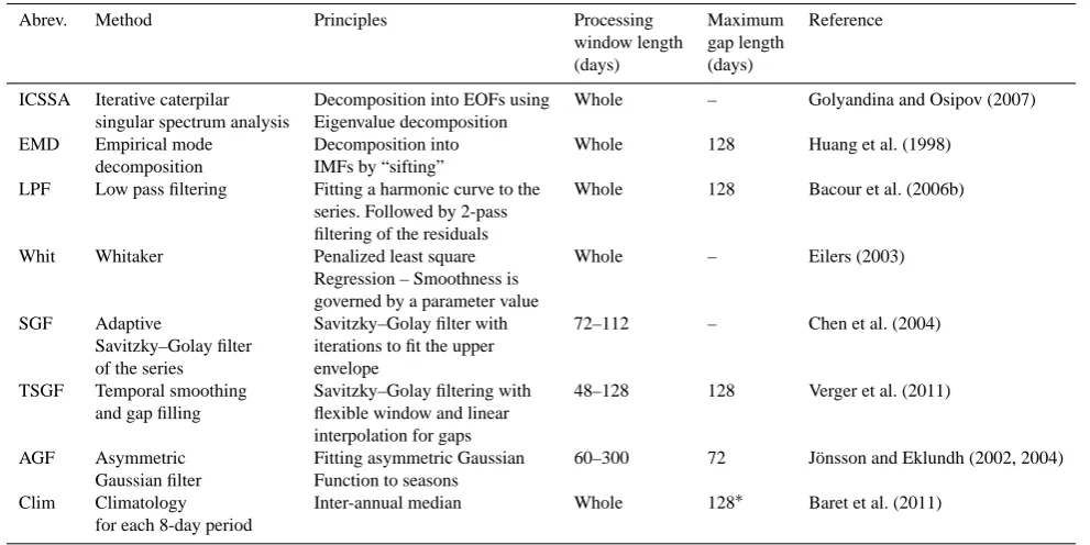
Table 1. List of the methods investigated. Length of processing window (whole means that the processing window is the whole time series) and maximum gap length tolerated are indicated.

Abrev. Method Principles Processing Maximum Reference

window length gap length (days) (days)

ICSSA Iterative caterpilar Decomposition into EOFs using Whole – Golyandina and Osipov (2007) singular spectrum analysis Eigenvalue decomposition

EMD Empirical mode Decomposition into Whole 128 Huang et al. (1998)

decomposition IMFs by “sifting”

LPF Low pass filtering Fitting a harmonic curve to the Whole 128 Bacour et al. (2006b) series. Followed by 2-pass

filtering of the residuals

Whit Whitaker Penalized least square Whole – Eilers (2003)

Regression – Smoothness is governed by a parameter value

SGF Adaptive Savitzky–Golay filter with 72–112 – Chen et al. (2004)

Savitzky–Golay filter iterations to fit the upper of the series envelope

TSGF Temporal smoothing Savitzky–Golay filtering with 48–128 128 Verger et al. (2011) and gap filling flexible window and linear

interpolation for gaps

AGF Asymmetric Fitting asymmetric Gaussian 60–300 72 J¨onsson and Eklundh (2002, 2004) Gaussian filter Function to seasons

Clim Climatology Inter-annual median Whole 128∗ Baret et al. (2011)

for each 8-day period

∗_{The maximum gap length applies on the yearly reconstructed time series, not on the original time series.}

requires 2 parameters: the window length and the number of eigenvectors (orthogonal functions) used for the reconstruc-tion. Better reconstruction can be obtained for large number of eigenvectors but at the cost of a decrease in the smooth-ness. After trial and error, the number of eigenvector was set to 1, and the window length was set to 40 days. This method allows filling gaps and forecasting data at the extremities of the time series.

Empirical mode decomposition method (EMD). This method proposed by Huang et al. (1998) consists in decom-posing the time series into a small number of intrinsic mode frequencies (IMFs) derived directly from the time series it-self using an adaptive iterative process where the data are represented by intrinsic mode functions, to which the Hilbert transform can be applied. The method requires setting 2 pa-rameters: the threshold for convergence and the maximum number of IMFs. The threshold for convergence is set to 0.3 according to Huang et al. (1998) and the maximum number of IMFs was restricted to 10 after trial and error. The first IMF, mostly affected by noise, was smoothed using a uni-form mean kernel to remove the high frequency fluctuations at the expense of a loss in the amplitude (Demir and Erturk, 2008). Note that the EMD method requires the time series to be continuous. To allow the application of EMD to MODIS time series, the missing data within 128 days were filled by linear interpolation as proposed by Verger et al. (2011). How-ever, when the time series contains gaps longer than 128 days, the whole series was not reconstructed. As a matter

of fact, linear interpolation provides generally poor perfor-mances in case of long periods without observations.

Low pass filtering (LPF). This method originally pro-posed by Thoning et al. (1989) was adapted by Bacour et al. (2006b) for better retrieving the seasonality from AVHRR time series. A time dependent function with 10 terms (2 poly-nomial and 8 harmonic terms) is first adjusted to the data. Then, the residuals of this first fitting are filtered with a low pass filter using two cut-off frequencies defined to separate the intra-annual and inter-annual variations. The final recon-struction is obtained by summing the polynomial and har-monic terms with the filtered residuals. Although this method may also be considered to be based on curve fitting, it applies over the time series as a whole. This method requires the data to be continuous. Hence, similarly to the EMD method, the gaps within 128 days were filled by linear interpolation. For gaps longer than 128 days, LPF was considered unsuccessful and, in this case, it results in missing reconstructed values for the whole time series.

depends on the data. After trial and error the smoothing pa-rameter was set to 100. The smoothness is also controlled by the order of differentiation which is fixed to 3 as proposed by Eilers (2003) for time series data sampled at regular intervals but with missing observations.

Adaptive Savitzky–Golay filter (SGF). This method pro-posed by Chen et al. (2004) iteratively applies the Savitzky– Golay filter (Savitzky and Golay, 1964) to match the upper envelope of the time series. This specific adaptation was de-signed to minimize the effects of cloud and snow contam-ination that generally decreases the estimates of vegetation indices such as NDVI as well as biophysical variables such as LAI. The original Savitzky–Golay filter consists in a lo-cal polynomial fitting with two parameters: the length of the temporal window used and the order of the polynomial. As proposed by Chen et al. (2004), the values of these parame-ters were optimized for each case to get the best match be-tween observations and reconstructed values. However, the range of variation of the window length was restricted to 72–112 days, and that of the polynomial order to 2–4. Miss-ing data in the time series were filled by linear interpolation independently of the size of the gaps as proposed in the orig-inal version.

Temporal smoothing and gap filling (TSGF). This method is another adaptation of the Savitzky–Golay filter where the polynomial degree was fixed to 2 but the temporal window may be asymmetric and variable in length. It was designed by Verger et al. (2011) to better handle time series with miss-ing observations. The temporal window correspondmiss-ing to a nominal date is adjusted to include at least 3 observations within a maximum 64 days period on each side of the nom-inal date. If less than 6 observations are available within the maximum±64 days temporal window, the polynomial fitting is not applied. The gaps in the reconstructed data are filled by an iterative (2 iterations) linear interpolation within 128 days window. For periods with missing data longer than 128 days, the interpolation is not applied which results in miss-ing data. The possible flattenmiss-ing of the reconstructed time series observed over peaks was further corrected by scaling the smoothed series to the observations in a local window (Verger et al., 2011).

Asymmetric Gaussian fitting (AGF). This method has been proposed by J¨onsson and Eklundh (2002, 2004) within the TIMESAT toolbox. A Gaussian function is adjusted locally over the growing and senescing parts of each season. The functions are finally merged to get a smooth transition from one season to another. This method can handle small gaps. The original TIMESAT implementation of this method in-cluded 3 conditions preventing the near-constant and noisy data from being processed. Two of these conditions (mini-mum seasonality in the data and maxi(mini-mum fraction of miss-ing data of 25 %) were not considered here to enlarge its do-main of validity in case of missing data. This thus allows more rigorous comparison with the other methods. However, the last condition was kept: the method was not applied over

seasons with gaps longer than 72 days and, in these cases, reconstructions for the entire time series are not provided.

Climatology (Clim). The climatology describes the typical yearly time course. It was included within the set of meth-ods investigated since it may provide smooth and complete time series with, however, no changes from year to year. The climatology was computed every 8 days during a year by av-eraging the values available over a±12 day window across all the years of the time series. The climatology was then corrected to provide more continuous and consistent tempo-ral patterns as proposed in Baret et al. (2011). To provide smoother values, a simple Savitzky–Golay filter was applied (Savitzky and Golay, 1964). Note that the climatology may present missing values when no observations in the 24 day temporal window centered on a given date in the year were available across, the years of the time series. In such situa-tions, linear interpolation was used to fill gaps shorter than 128 days. Gaps longer than 128 days will result in missing data. Once the average yearly time course was computed, it was replicated across all the years considered to provide a reconstructed time series.

2.3 Evaluation approach

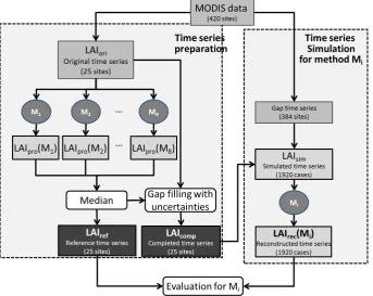
The approach proposed to evaluate the methods is based on two steps as sketched in Fig. 1. The first one is dedicated to the preparation of reference time series over a limited number of representative sites. As a result of this step, two time series will be output: (i) a time series with no gaps and small uncer-tainties considered as the reference (LAIref), and (ii) a time series with no gaps with realistic uncertainties (LAIcomp). In the second step, time series with variable occurrence of missing data will be simulated (LAIsim)from the previously LAIcomp time series. Each method will be applied on this LAIsim data to get the corresponding reconstructed time se-ries (LAIrec). Finally, the LAIrec obtained with each of the 8 methods will be evaluated based on a range of metrics de-scribing the fidelity, the roughness of time series and the ac-curacy of phenological stages that can be derived from the time series.

2.3.1 Generation of the reference and completed LAI time series.

Fig. 1. Flow chart describing the approach used. Mi corresponds to methodiwithin the 8 investigated. LAIrec(Mi)corresponds to the reconstructed time series based on methodMi.

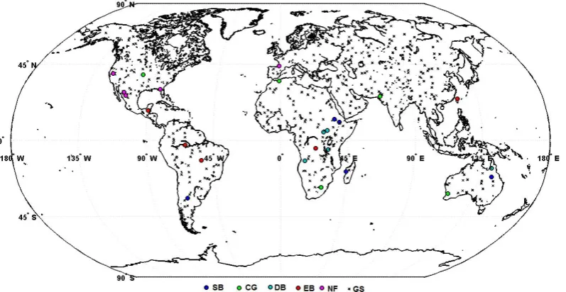
and NF sites, most sites show significant fraction of miss-ing data. The 5 sites showmiss-ing the minimal gap fraction with a large variability in seasonal patterns were finally selected. The same process was applied to SB, GC and EB classes, re-sulting in a total of 25 sites (5 sites for each of the 5 biome classes) (Table 2, Fig. 2)

The eight methods presented earlier were applied to each of the 25 sites and show very good agreement. The median across all methods is a good approximation of the expected LAI product values (Fig. 3) with 4 out of the 8 methods in-vestigated very close (RMSE (root mean square error) lower than 0.05) to the median across all methods. The time series made with the median across the 8 methods will therefore be considered as the reference values, LAIref, in the following. This LAIref does not show any missing data since the gaps in the original time series were filled by the reconstructed values of the 8 methods. LAIrefconstitutes a good reference with minimal uncertainties attached to the LAI values be-cause of the temporal smoothing coming from each method and the computation of the median across the 8 methods. A second set of time series was generated to provide realistic LAI values: the LAIori were complemented at the location of missing data by LAIref values contaminated by a noise that was randomly drawn within the distribution of residuals (LAIref-LAIori)for each site. These realistic but continuous temporal profiles with no gaps (LAIcomp)will be used in the

second step of the approach for simulating time series with gaps.

2.3.2 Simulation of time series with gaps

Fig. 2. Location of the 25 sites being selected (◦) (Table 2) and the 384 sites used to simulate gaps in the data (×). SB: shrub savannah bare, GC: crop grassland, DB: deciduous broadleaf forests, EB: evergreen broadleaf forests, NF: needleleaf forests.

Table 2. Sites selected for the study for the 5 biomes. The site num-ber in BELMANIP2 ensemble of 420 sites, latitude and longitude and fraction of missing data (% gap) are indicated.

Biome Site # Lat.(◦) Lon. (◦) % gap

Shrub Savannah 5 −34.02 −65.63 1

Bare (SB) 136 −18.46 44.41 3

176 12.49 36.34 2

186 10.70 39.41 1

293 −21.54 143.83 1

Crop Grassland 69 38.63 −98.91 5

(GC) 127 −27.61 27.95 1

225 35.09 −1.00 1

280 −31.38 116.87 1

338 25.99 68.52 0

Deciduous Broadleaf 131 −11.99 16.43 11

forests (DB) 146 −5.45 31.74 9

162 4.86 28.80 8

165 5.98 31.18 1

296 −16.45 142.62 1

Evergreen Broadleaf 19 −11.75 −53.35 41

Forests (EB) 30 −2.68 −63.65 48

50 17.59 −89.78 45

142 −4.60 23.44 38

320 24.54 121.25 41

Needleleaf Forests 54 28.39 −108.25 11

(NF) 55 26.53 −106.68 13

62 39.49 −120.83 18

65 30.28 −83.85 16

244 43.86 −1.10 20

Table 3. Number of sites per vegetation class in BELMANIP2 set of sites, and number of cases considered in the gap simulation ex-periment.

Vegetation class SB CG DB EB NF Total

Nb. sites in

144 123 35 36 46 384

BELMANIP2 Nb. cases (time

720 615 175 180 230 1920 series) simulated

A total of 384 sites were used to simulate the gaps in the data (Table 3). Because each vegetation class is represented by 5 sites used for the LAIrefand LAIcompvalues, a total of 1920 cases (384×5) with realistic LAI uncertainties and gap structure were finally available.

2.4 Metrics used to quantify performances

Fig. 3. Comparison between the original LAI values (LAIori)and the median of the reconstructed values (LAI_ref) based on the 8 methods considered over the 25 selected sites (Table 2, Fig. 2) (N=7561;R2=0.90; RMSE=0.231; Bias= −0.008). The col-ors of this density plot correspond to the frequency of data in each of the 0.1×0.1 cells LAI values.

2.4.1 Metrics based on LAI values

The RMSE (root mean square error) computed over all cases quantifies the fidelity of the reconstruction of the time series:

RMSE= v u u u t

PN j=1

Pnj t=1

LAIjrec(t )−LAIj_ref(t )

2

PN j=1nj

, (1)

where LAIj_ref(t )and LAIjrec(t )are, respectively, the reference and the reconstructed values for datet and casej,nj is the number of dates with observations for casej andN is the number of cases considered.

Finally, the metrics proposed by Whittaker (1923) called here roughness will be used to quantify the shaky nature of the reconstructed time series:

Roughness= v u u u t

PN

j=1 Pnj

t=1

LAIjrec(t )−LAI

j

rec(t−1) 2

PN j=1nj

. (2)

2.4.2 Metrics based on phenology

The 5 evergreen broadleaf forest sites were excluded from these metrics since the identification of seasonality was ques-tionable at the single pixel scale considered in this study, and would result in large uncertainties in the timing of pheno-logical stages if they exist (some sites do not show obvious seasonality). Three phenological events were considered: the start of season (SoS), maximum of season (MoS) and end of season (EoS). SoS and EoS were defined similarly to J¨onsson and Eklundh (2002) as the timing when LAI reaches 20 %

Fig. 4. Cumulated distribution of the fraction of missing data (% gap) in the simulated time series (LAI_sim)for each of the 5 veg-etation classes (SB, CG, DB, EB, NF).

of the whole LAI amplitude before (SoS) or after (EoS) the timing of maximum LAI (MoS). The reference dates of these three stages were derived by applying this phenology extrac-tion method to the LAIrefdata (Pref). Then the RMSE for the timing of SoS, MoS and EoS are computed:

RMSE (days)= v u u u t

PN j=1

Pmj s=1

Precj (s)−Prefj (s)

2

PN j=1mj

, (3)

whereP_refj (s)andPrecj (s)are, respectively, the reference and the reconstructed dates for the phenological events and case j,mjis the number of phenological events for casej(i.e. the number of seasons in the time seriesj andN is the number of cases considered).

3 Results

The methods will first be evaluated with regards to fidelity and roughness of the reconstructed time series. Then, they will be evaluated with regard to their ability to describe the phenology. In both the cases, the impact of the occurrence of missing data (% gap) and the length of gaps (LoG), i.e. the number of days between two consecutive valid observations, will be analyzed.

3.1 Performances for LAI reconstruction

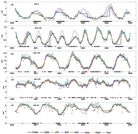
Fig. 5. Time series (LAIrec)reconstructed by the several methods in presence of medium occurrence of missing data (25 %<% gap<35 %). Black dots correspond to LAIcompat the location of observations. Empty circles on the x-axis correspond to the dates of missing data. The dashed black curve corresponds to LAIref. Note that because of the structure of missing data, EMD, LPF and AGF were not reconstructed for sites 5 and 65, as well as AGF for site 338.

within the 1920 ones have been selected (Fig. 5) and their temporal profiles plotted against LAIref. They represent the 5 typical vegetation types under a medium occurrence of missing data. Visual inspection shows that

– The climatology is often shifted from the reference

tem-poral profile, highlighting the inter-annual fluctuations, particularly for non-forest vegetation types (SB and CG in Fig. 5).

– In presence of periods with long and continuous missing

data, several methods were not able to reconstruct the time series over these periods, particularly TSGF and Clim, while AGF, EMD, LPF fail for the entire time se-ries (SB in Fig. 5). However, the other methods (ICSSA, Whit, SGF) showing continuity in LAIrecdo not always provide realistic (as compared with LAIref) reconstruc-tions in such cases.

– When observations show a significant level of temporal

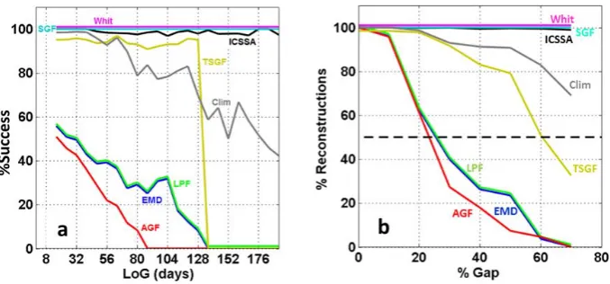
Fig. 6. (a) Fraction of gaps reconstructed (% success) as a function of the length of the gaps (LoG). (b) Fraction of dates reconstructed (% reconstructions) as a function of the % gap. The horizontal dashed line represents the 50 % threshold of % reconstructions. The several methods are represented by different colors. Some values were slightly shifted vertically to ease the reading when curves were overlapping.

both in terms of fidelity (closeness to LAIref)and rough-ness, particularly for SGF and EMD.

3.1.1 Capacity to reconstruct the temporal series in presence of missing data

All the methods were not able to fill all of the gaps, i.e. to provide an estimated value in gaps. This was quantified by the % success, i.e. the fraction of gaps that were able to be filled. Whit, SGF, ICSSA allow to fill most of the gaps even if they are very long (Fig. 6a). Conversely, EMD, LPF and AGF show a rapid decrease of %Success with the length of the gaps, with no reconstructions for gaps longer than 88 (AGF) to 136 days (EMD, LPF). Even for small gaps, only 50 % of them were filled. This is due to the fact that a specific gap may be associated to other ones in a close vicinity in the time series. TSGF is able to fill gaps up to gap length of 128 days as expected by its definition. The climatology shows also a progressive decrease of % success with gaps of 128 days length being filled in 80 % of cases because of the accumulation of observations over the 9 yr period.

The capacity to fill individual gaps has consequences on the reconstruction fraction (% reconstructions), i.e. the frac-tion of dates with reconstructed LAI values, LAIrec, relative to the total number of dates in the LAIcomptime series. Only three methods (Whit, SGF, ICSSA) were able to provide a continuous reconstructed time series over all the cases inves-tigated (Fig. 6b) even for large occurrence of missing data in agreement with Fig. 6a. In contrast, AGF is characterized by the smallest %Success (Fig. 6a) and % reconstruction (Fig. 6b): only 50 % of the dates are reconstructed for cases with more than 25 % of missing data in their time series (Fig. 6b). LPF and EMD that do not accept gaps longer than 128 days (Table 1) show also a similar drastic decrease of the reconstruction fraction with the occurrence of missing data in the cases considered (Fig. 6b). The TSGF method, although also not filling gaps longer than 128 days is more

resilient to the occurrence of gaps: TSGF was able to recon-struct more than 50 % of the data for cases with more than 60 % of missing data. When a gap longer than 128 days ap-pears in a time series, the remaining parts of the time series are reconstructed. This was not the case for LPF and EMD for which the whole time series was not reconstructed for cases having a gap longer than 128 days. Clim allows for the reconstruction of most time series, even for cases with large amounts of missing data, benefiting from the replications be-tween years, cloudy days being not always the same day of the year.

To improve the robustness of the metrics used to character-ize the performances on LAI and phenology reconstruction they will be computed only when % reconstructions>50 % (Fig. 6b). As a consequence, all the methods will be compared for cases with less than % gap<20 %; TSGF, Clim, ICSSA, SGF and Whit will be compared for 20 %<% gap<60 %; and for % gap>60 %, only Clim, IC-SSA, SGF and Whit will be compared (Fig. 6b).

3.1.2 Fidelity to LAIref

Fig. 7. RMSE as a function of % gap. The RMSE is computed be-tween LAIrefand the reconstructed LAIrectime series over dates with actual observations in LAIsim. The values were slightly shifted vertically to ease the reading when curves were overlapping.

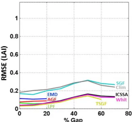
Over dates of missing observations, the reconstruction ca-pacity degrades rapidly as a function of the length of gaps for all methods except Clim that keeps a RMSE value around 0.35 independent from the expected gap length (Fig. 8a). LPF and TSGF provide the best performances up to gap length around 100 days when Clim starts to be the best method. AGF, Whit EMD and SGF show similar performances with RMSE lower than the climatology up to gap length around 70 days, while ICSSA performances rapidly degrade with the length of gaps. The fidelity of reconstructions in gaps as a function of the fraction of missing observations in the time series (Fig. 8b) derives logically from the reconstruc-tion performances as a funcreconstruc-tion of the gap length (Fig. 8a). The RMSE values computed over dates of missing observa-tions are relatively low for all methods up to % gap<20 %. Then SGF, Whit and ICSSA show a rapid increase of the RMSE with % gap with poorer performances as compared to Clim for % gap>30 % (Fig. 8b). These three methods show obvious artifacts when reconstructing long gaps (Fig. 5, non-forest sites 5 and 338). TSGF shows relatively low RMSE values up to 60 % gap (Figs. 7, 8b). Clim shows similar per-formances over dates with missing data (Fig. 8b) and dates with observations (Fig. 7) as expected since it is not depen-dent on the local observations.

3.1.3 Roughness

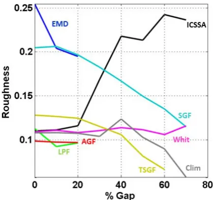
The roughness was computed over the whole reconstructed time series and is presented as a function of % gap (Fig. 9). Results show that for % gap<30 %, EMD and SGF show the highest roughness values in agreement with the previous qualitative observations (Fig. 5). The behavior of SGF is

con-trolled by its iterative nature that puts emphasis on fidelity (relative to the upper envelope). For EMD, the 10 modes se-lected were showing variable patterns and it was difficult to find a better compromise between smoothness and fidelity. ICSSA shows a roughness value close to that of Clim for % gap<20 %. However, the roughness of ICSSA strongly increases when % gap> 20 %. This is partially due to in-consistencies observed in its temporal pattern with abrupt variations in the periods with high discontinuities in the data (Fig. 5, jumps observed between the lowest and the highest values when data are missing for non-forest sites 5 and 338). AGF and LPF show the smoothest temporal profiles how-ever limited to cases with % gap<20 %. Whit provides al-ways smooth reconstructed profiles, even for large amount of missing data. This is obviously controlled by the smoothing parameter. Whit is just slightly rougher than LPF and AGF. TSGF shows a slightly higher roughness values than Whit for the % gap<30 %, with a significant decrease when % gap in-creases. This is due to the linear interpolation used to fill the gaps that explains also the decrease of roughness for EMD, SGF and Clim when % gap increases.

3.2 Performances for describing the phenology

The capacity of the several methods to identify the main phe-nological stages (SoS, MoS and EoS) was evaluated using the dates derived from LAIrefas a reference. The performances (RMSE in days) were analyzed as a function of the occur-rence of missing data (% gap). Results show a general degra-dation of RMSE when % gap increases for the three stages considered.

Fig. 8. RMSE as a function of the length of gaps (a) and fraction of missing observations (% gap ) (b). The RMSE is computed between LAIrefand the reconstructed LAIrectime series over dates with missing observations in LAIsim.

Fig. 9. Roughness of LAIrecas a function of % gap in LAIsim.

4 Discussion and conclusion

This study compares 8 methods designed to improve the con-tinuity and consistency of time series by filling gaps cre-ated by missing observations and smoothing the temporal profiles to reduce local uncertainties. However, the perfor-mances of the different methods for processing time series depend on their implementation (e.g. very different results with two variants of Savitzky–Golay filter: SGF and TSGF). The selected methods were applied here as close as possi-ble to their standard implementation including the original parameterization as proposed by their authors. When the pa-rameters for each method were not known they were adjusted using a trial and error approach. Other techniques based on systematic cross validation could have been implemented. This was not considered here since it would lead to signif-icant increase in computation time not compatible with

cur-rent operational processing lines capabilities. The time series considered correspond to actual MODIS LAI products over a sample of sites that were selected to be both representative of the diversity of seasonal patterns and of the distribution of the missing observations. This approach was expected to improve the realism of the context of the analysis that ac-counts for the implicit links between the vegetation type and the distribution of missing observations. This may be critical for filling gaps or smoothing the time series. The approach allowed defining a set of reference time series used to quan-tify the accuracy of each of the 8 methods as a function of the fraction of missing observations.

Results clearly show that some methods including LPF, AGF and EMD were failing in about 50 % of the situations when the fraction of missing observations was larger than 20 % which represents about 60 % of the situations investi-gated here. This is partly due to the principles on which these methods are based, but also partly to their implementation. Consequently, great care should be taken with the implemen-tation of such methods to improve their rate of applicability in case of significant periods with missing observations. Con-versely, ICSSA, Whit and Clim methods were applicable in almost all situations while TSGF shows intermediate behav-ior.

Fig. 10. RMSE relative to the timing (in days) of the start of season (a), maximum of season (b) and end of season (c). The RMSE is evaluated between the phenological dates computed with LAIrefand those derived from the reconstructed LAIrectime series using the several methods investigated.

Fig. 11. RMSE as a function of Roughness observed over the reconstructed times series using the several methods. Color dots correspond to the values for the different methods over the 25 sites for cases with % gap in the selected classes of occurrence of missing data: 0–15 % (a) and 45–55 % (b). Note that EMD, LPF and AGF are only displayed for the lowest occurrence of missing data (0 %<% gap<15 %). Black circles correspond to LAIcompand black diamonds to LAIref. Lines correspond to the zero-offset linear regressions.

adaptive temporal window, although limited to gaps smaller than 128 days. For longer periods without observations, the Clim method appears to be the best one provided that enough data are available over the time series of years used to build the climatology. Note that the reconstruction performances for the best methods and for gaps shorter than 100 days ful-fills the GCOS criterion on LAI uncertainties (RMSE≤0.5) (GCOS, 2010) although the reconstruction uncertainty is only part of the error budget

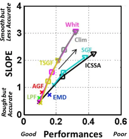
Each method is based explicitly (Whit) or implicitly (the other methods) on a balance between fidelity and rough-ness. This is clearly demonstrated when plotting Rough-ness and RMSE performances for each of the 25 selected sites (Table 2, Fig. 2) for a class of occurrence of miss-ing data (Fig. 11). For each method, all the 25 sites are ap-proximately organized around a line passing through the ori-gin. The slope of this line indicates the balance between fi-delity and roughness. For relatively continuous time series (0 %<% gap<15 %), TSGF, ICSSA and Whit focus more on fidelity than smoothness (Fig. 11a). Conversely, LPF,

EMD and AGF are focusing more on smoothness than fi-delity. SGF constitutes a particular case because the fidelity is targeting the upper envelope of the points, resulting in larger RMSE values, while roughness is also quite important as described previously. Clim provides the steepest slope, with smooth temporal profiles but a loose match with ob-servations. Note that the slope of Clim is in between that of LAIcomp and LAIref(for which RMSE was replaced by the standard deviation between observations). For the larger oc-currence of missing data (Fig. 11b), the slopes increase sig-nificantly due to an increase of RMSE mostly due to inaccu-rate reconstructions in the gaps, and a decrease of roughness due to more simple patterns in the observations, except for ICSSA as noticed earlier.

Fig. 12. Performances (distance to the origin) and slopes in the (Roughness, RMSE) feature plane (Fig. 11) associated to each method for 0 %<% gap≤15 % (×), 25 %<% gap≤35 % () and 35 %<% gap≤45 % (∇). Note that EMD, LPF and AGF are only displayed for the lowest % gap class. The black arrow indicates the effect of an increase of the fraction of missing data.

considered: the closer to the origin (0,0), the smoother and the better match with LAIref (low RMSE). The behavior of each method as a function of the occurrence of missing data is well sketched in the (performances, slopes) feature plane (Fig. 12). For low amounts of missing data, all the methods provide good performances except SGF and Clim for the rea-sons exposed previously. When the fraction of missing data increases, each method follows a particular pattern (the black arrow in Fig. 12) with a degradation of the performances and an increase in the slope indicating more emphasis on the smoothness of the temporal profiles through a reduction of the roughness. For medium and high occurrence of missing data, TSGF provides clearly the best overall performances although restricted to gaps smaller than 128 days, followed by Whit. SGF and ICSSA show poor performances.

The consequences of the application of the several time se-ries processing methods on their capacity to describe phenol-ogy characteristics were finally evaluated. As expected, the methods providing the best accuracy on LAI estimation were also more accurate for dating specific phenological events such as start, maximum and end of season (Fig. 13).

The effect of gaps on the derivation of time series appears as a major limitation of the accuracy of the reconstructed temporal profiles. Techniques based on the processing of the time series as a whole (ICSSA, EMD, LPF, Whit and Clim) were not demonstrated to perform systematically better than techniques based on a limited temporal window (AGF, SGF,

Fig. 13. Accuracy of the start of season retrieval expressed in RMSE (days) as a function of the accuracy of LAI estimated expressed in RMSE. The same colors (corresponding to methods) and markers (corresponding to classes of % gap) as in Fig. 12 are used.

TSGF) although they were expected to fill long gaps with the “experience” gained across the several years available in the time series. Local methods were generally more faithful but were lacking capacity to fill long gaps. Most methods were performing poorer than Clim to gaps longer than about 100 days. Future works should therefore be dedicated to develop methods where the features derived from the exploitation of the several years available in the time series including the cli-matology, could be injected more explicitly as a background information for improving the reliability of methods work-ing over a limited time window, such as a season or part of it, with emphasis on the capacity to provide accurate pheno-logical timing as proposed in Verger et al. (2013).

Acknowledgements. This research has received funding from the Geoland2 European Community’s Seventh Framework Program (FP7/2007-2013) under grant agreement no. 218795. A. Verger was funded by the VALi+d and Juan de la Cierva postdoctoral programs. Many thanks also to the MODIS teams who made available to the wide community the LAI data used in this study.

References

Alcaraz-Segura, D., Liras, E., Tabik, S., Paruelo, J., and Cabello, J..: Evaluating the Consistency of the 1982–1999 NDVI Trends in the Iberian Peninsula across Four Time-series Derived from the AVHRR Sensor: LTDR, GIMMS, FASIR, and PAL-II, Sensors, 10, 1291–1314, 2010.

Atkinson, P. M., Jeganathan, C., Dash, J., and Atzberger, C.: Inter-comparison of four models for smoothing satellite sensor time-series data to estimate vegetation phenology, Remote Sens. Env-iron., 123, 400–417, 2012.

Azzali, S. and Menenti, M.: Mapping isogrowth zones on continen-tal scale using temporal Fourier analysis of AVHRR-NDVI data, Int. J. Appl. Earth Obs., 1, 9–20, 1999.

Bacour, C., Baret, F., B´eal, D., Weiss, M., and Pavageau, K.: Neural network estimation of LAI, fAPAR, fCover and LAIxCab, from top of canopy MERIS reflectance data: principles and validation, Remote Sens. Environ., 105, 313–325, 2006a.

Bacour, C., Br´eon, F.-M., and Maignan, F.: Normalization of the directional effects in NOAA-AVHRR reflectance measurements for an improved monitoring of vegetation cycles, Remote Sens. Environ., 102, 402–413, 2006b.

Baret, F., Morissette, J., Fernandes, R., Champeaux, J. L., My-neni, R., Chen, J., Plummer, S., Weiss, M., Bacour, C., Gar-rigue, S., and Nickeson, J.: Evaluation of the representative-ness of networks of sites for the global validation and inter-comparison of land biophysical products. Proposition of the CEOS-BELMANIP, IEEE T. Geosci. Remote, 44, 1794–1803, 2006.

Baret , F., Hagolle, O., Geiger, B., Bicheron, P., Miras, B., Huc, M., Berthelot, B., Weiss, M., Samain, O., Roujean, J. L., and Leroy, M.: LAI, fAPAR and fCover CYCLOPES global products derived from VEGETATION. Part 1: Principles of the algorithm, Remote Sens. Environ., 110, 275–286, 2007.

Baret, F., Weiss, M., Verger, A., and Kandasamy, S.: BioPar Meth-ods Compendium - LAI, FAPAR and FCOVER from LTDR AVHRR series. Report for EC contract FP-7-218795, avail-able at: http://www.geoland2.eu/portal/documents/CA80C881. html, INRA-EMMAH, Avignon, p. 46, 2011.

Beck, P. S. A., Atzberger, C., Hogda, K. A., Johansen, B., and Skid-more, A. K.: Improved monitoring of vegetation dynamics at very high latitudes: A new method using MODIS NDVI, Remote Sens. Environ., 100, 321–334, 2006.

Becker-Reshef, I., Vermote, E., Lindeman, M., and Justice, C.: A generalized regression-based model for forecasting winter wheat yields in Kansas and Ukraine using MODIS data, Remote Sens. Environ., 114, 1312–1323, 2010.

Berterretche, M., Hudak, A. T., Cohen, W. B., Maiersperger, T. K., Gower, S. T., and Dungan, J.: Comparison of regression and geostatistical methods for mapping Leaf Area Index (LAI) with Landsat ETM+data over a boreal forest, Remote Sens. Environ., 96, 49–61, 2005.

Boles, S. H., Xiao, X., Liu, J., Zhang, Q., Munkhtuya, S., Chen, S., and Ojima, D.: Land cover characterization of Temperate East Asia using multi-temporal VEGETATION sensor data, Remote Sens. Environ., 90, 477–489, 2004.

Borak, J. S. and Jasinski, M. F.: Effective interpolation of incom-plete satellite-derived leaf-area index time series for the conti-nental United States, Agr. Forest Meteorol., 149, 320–332, 2009.

Camacho, F., Cernicharo, J., Lacaze, R., Baret, F., Weiss, M.: GEOV1: LAI, FAPAR essential climate variables and FCOVER global time series capitalizing over existing products. Part 2: Validation and intercomparison with reference products, Remote Sensing of Environment, available online 29 March 2013, ISSN 0034-4257, doi:10.1016/j.rse.2013.02.030, 2013

Chen, J. M. and Black, T. A.: Defining leaf area index for non-flat leaves, Plant Cell Environ., 15, 421–429, 1992.

Chen, J., J¨onsson, P., Tamura, M., Gu, Z., Matsushita, B., and Ek-lundh, L.: A simple method for reconstructing a high quality NDVI time series data set based on the Savitzky-Golay filter, Re-mote Sens. Environ., 91, 332–344, 2004.

Coops, N. C., Wulder, M. A., and Iwanicka, D.: Large area mon-itoring with a MODIS-based Disturbance Index (DI) sensitive to annual and seasonal variations, Remote Sens. Environ., 113, 1250–1261, 2009.

Defourny, P., Bicheron, P., Brockmann, C., Bontemps, S., Van Bo-gaert, E., Vancutsem, C., Pekel, J.F., Huc, M., Henry, C., Ran-era, F., Achard, F., di Gregorio, A., Herold, M., Leroy, M., and Arino, O.: The first 300 m global land cover map for 2005 using ENVISAT MERIS time series: a product of the GlobCover sys-tem, Proceedings of the 33rd International Symposium on Re-mote Sensing and Environment, Stresa, Italy, 1–4, 2009. De Kauwe, M. G., Disney, M. I., Quaife, T., Lewis, P., and Williams,

M.: An assessment of the MODIS collection 5 leaf area index product for a region of mixed coniferous forest, Remote Sens. Environ., 115, 767–780, 2011.

Demir, B. and Erturk, S.: Empirical mode decomposition pre-process for higher accuracy hyperspectral image classification, IGRARSS. IEEE, Boston (USA), II, 939–941, 2008.

Deng, F., Chen, J. M., Chen, M., and Pisek, J.: Algorithm for global leaf area index retrieval using satellite imagery, IEEE T. Geosci. Remote, 44, 2219–2229, 2006.

Dente, L., Satalino, G., Mattia, F., and Rinaldi, M.: Assimilation of leaf area index derived from ASAR and MERIS data into CERES-Wheat model to map wheat yield, Remote Sens. Envi-ron., 112, 1395–1407, 2008.

Eilers, P. H. C.: A Perfect Smoother, Anal. Chem., 75, 3631–3636, 2003.

Fang, H., Liang, S., Townshend, J. R., and Dickinson, R. E.: Spa-tially and temporally continuous LAI data sets based on an inte-grated filtering method: Examples from North America, Remote Sens. Environ., 112, 75–93, 2008.

Ganguly, S., Schull, M. A., Samanta, A., Shabanov, N. V., Milesi, C., Nemani, R. R., Knyazikhin, Y., and Myneni, R. B.: Gener-ating vegetation leaf area index earth system data record from multiple sensors. Part 1: Theory, Remote Sens. Environ., 112, 4333–4343, 2008.

Gao, F., Morisette, J., Wolfe, R. E., Ederer, G., Pedelty, J., Masuoka, E. J., Myneni, R., Tan, B., Nightingale, J. M.: An algorithm to produce temporally and spatially continuous MODIS LAI time series, IEEE Geosci. Remote Sens. Lett., 5, 60–64, 2008. GCOS: GCOS-107, Supplemental details to the satellite based

com-ponent of the “implementation plan for the global observing sys-tem for climate in support of the UNFCCC”, GCOS/WMO, Gen-eve (Switzerland), p. 103, 2006.

Golyandina, N. and Osipov, E.: The “Caterpillar”-SSA method for analysis of time series with missing values, J. Stat. Plan. Infer., 137, 2642–2653, 2007.

Goovaerts, P.: Geostatistics for natural resources evaluation, New York, Oxford University Press, 1997.

Hansen, M. C., DeFries, R. S., Townshend, J. R. G., Sohlberg, R., Dimiceli, C., and Carroll, M.: Towards an operational MODIS continuous field percent tree cover algorithm: examples using AVHRR and MODIS data, Remote Sens. Environ., 83, 303–319, 2002.

Hansen, M. C., Shimabukuro, Y. E., Potapov, P., and Pittman, K.: Comparing annual MODIS and PRODES forest cover change data for advancing monitoring of Brazilian forest cover, Remote Sens. Environ., 112, 3784–3793, 2008.

Heiskanen, J. and Kivinen, S.: Assessment of multispectral, -temporal and -angular MODIS data for tree cover mapping in the tundra-taiga transition zone, Remote Sens. Environ., 112, 2367– 2380, 2008.

Hird, J. N. and McDermid, G. J.: Noise reduction of NDVI time series: An empirical comparison of selected techniques. Remote Sens. Environ., 113, 248–258, 2009a.

Hird, J. N. and McDermid, G. J.: Noise reduction of NDVI time series: An empirical comparison of selected techniques, Remote Sens. Environ., 113, 248–258, 2009b.

Holben, B. N.: Characteristics of maximum-value composite im-ages from temporal AVHRR data, Int. J. Remote Sens., 7, 1417– 1434, 1986.

Huang, N. E., Shen, Z., Long, S. R., Wu, M. C., Shih, H. H., Zheng, Q., Yen, N.-C., Tung, C. C., and Liu, H. H.: The empirical mode decomposition and the Hilbert spectrum for nonlinear and non-stationary time series analysis, P. R. Soc. Lond. A Mat., 454, 903–995, 1998.

Jakubauskas, M. E., Legates, D. R., and Kastens, J. H.: Crop iden-tification using harmonic analysis of time series AVHRR NDVI data, Computers Electronics in Agriculture, 37, 127–139, 2002. Jiang, B., Liang, S., Wang, J., and Xiao, Z.: Modeling MODIS LAI

time series using three statistical methods, Remote Sens. Envi-ron., 114, 1432–1444, 2010.

J¨onsson, P. and Eklundh, L.: Seasonality extraction by function-fitting to time series of satellite sensor data, IEEE T. Geosci. Re-mote, 40, 1824–1832, 2002.

J¨onsson, P. and Eklundh, L.: TIMESAT – a program for analyzing time series of satellite sensor data, Comput. Geosci., 30, 833– 845, 2004.

Kandasamy, S., Neveux, P., Verger, A., Buis, S., Weiss, M., and Baret , F.: Improving the consistency and continuity of MODIS 8 day leaf area index products, International Journal of Electronics and Telecommunications, 58, 141–146, 2012.

Kastens, J. H., Kastens, T. L., Kastens, D. L. A., Price, K. P., Mar-tinko, E. A., and Lee, R.-Y.: Image masking for crop yield fore-casting using AVHRR NDVI time series imagery, Remote Sens. Environ., 99, 341–356, 2005.

Kobayashi, H., Suzuki, R., and Kobayashi, S.: Reflectance season-ality and its relation to the canopy leaf area index in an eastern Siberian larch forest: Multi-satellite data and radiative transfer analyses, Remote Sens. Environ., 106, 238–252, 2007.

Ma, M. and Veroustraete, F.: Reconstructing pathfinder AVHRR land NDVI timeseries data for the Northwest of China, Adv. Space Res., 37, 835–840, 2006.

Martinez, B. and Gilabert, M. A.: Vegetation dynamics from NDVI time series analysis using the wavelet transform, Remote Sens. Environ., 113, 1823–1842, 2009.

Meroni, M., Atzberger, C., Vancutsem, C., Gobron, N., Baret, F., Lacaze, R., Eerens, H., and Leo, O.: A protocol for the evalua-tion of agreement between space remote sensing time series and application to SPOT-VEGETATION fAPAR products, Interna-tional Journal of Applied Observations and Geoinformation, 51, 1951–1962, 2013.

Moody, E. G., King, M. D., Platnick, S., Schaaf, C. B., and Gao, F.: Spatially complete global spectral surface albedos: Value-added datasets derived from Terra MODIS land products, IEEE T. Geosci. Remote, 43, 144–158, 2005.

Myneni, R. B., Hoffman, S., Knyazikhin, Y., Privette, J. L., Glassy, J., Tian, Y., Wang, Y., Song, X., Zhang, Y., Smith, G. R., Lotsch, A., Friedl, M., Morisette, J. T., Votava, P., Nemani, R. R., and Running, S. W.: Global products of vegetation leaf area and ab-sorbed PAR from year one of MODIS data, Remote Sens. Envi-ron., 83, 214–231, 2002.

Pettorelli, N., Vik, J. O., Mysterud, A., Gaillard, J.-M., Tucker, C. J., and Stenseth1, N. C.: Using the satellite-derived NDVI to as-sess ecological responses to environmental change, Trends Ecol. Evol., 20, 503–510, 2005.

Pinzon, J. E., Brown, M. E., and Tucker, C. J.: Satellite time series correction of orbital drift artifacts using empirical mode decom-position, in: EMD and its Applications, edited by: Huang, N. E. and Shen, S. S. P., World Scientific Publishers, Singapore, 167– 186, 2005.

Pouliot, D., Latifovic, R., Fernandes, R., and Olthof, I.: Evaluation of annual forest disturbance monitoring using a static decision tree approach and 250 m MODIS data, Remote Sens. Environ., 113, 1749–1759, 2009.

Qi, J. and Kerr, Y.: On current compositing algorithms, Remote Sensing Reviews, 15, 235–256, 1997.

Rouse, J. W., Haas, R. H., Schell, J. A., Deering, D. W., and Harlan, J. C.: Monitoring the vernal advancement of retrogradation of natural vegetation, NASA/GSFC, p. 371, 1974.

Savitzky, A. and Golay, M. J. E.: Smoothing and differentiation of data by simplified least square procedures, Anal. Chem., 36, 1627–1639, 1964.

Schubert, P., Eklundh, L., Lund, M., and Nilsson, M.: Estimating northern peatland CO2 exchange from MODIS time series data, Remote Sens. Environ., 1178–1189, 2010.

Shabanov, N. V., Huang, D., Yang, W., Tan, B., Knyazikhin, Y., My-neni, R. B., Ahl, D. E., Gower, S. T., and Huete, A. R.: Analysis and Optimization of the MODIS Leaf Area Index Algorithm Re-trievals Over Broadleaf Forests, IEEE T. Geosci. Remote Sens., 43, 1855–1865, 2005.

Thenkabail, P. S., Schull, M., and Turral, H.: Ganges and Indus river basin land use/land cover (LULC) and irrigated area mapping us-ing continuous streams of MODIS data, Remote Sens. Environ., 95, 317–341, 2005.

Thoning, K. W., Tans, P. P., and Komhyr, W. D.: Atmospheric carbon dioxide at Mauna Loa Observatory: 2. Analysis of the NOAA GMCC data, 1974–85, J. Geophys. Res., 94, 8549–8565, 1989.

and SPOT vegetation NDVI data, Int. J. Remote Sens., 26, 4485– 4498, 2005.

Verger, A., Baret, F., and Weiss, M.: Performances of neural net-works for deriving LAI estimates from existing CYCLOPES and MODIS products, Remote Sens. Environ., 112, 2789–2803, 2008.

Verger, A., Baret , F., and Weiss, M.: A multisensor fusion approach to improve LAI time series, Remote Sens. Environ., 115, 2460– 2470, 2011.

Verger, A., Baret, F., Weiss, M., Kandasamy, S., and Vermote, E.: The CACAO method for smoothing, gap filling and characteriz-ing anomalies in satellite time series, IEEE T. Geosci. Remote, 51, 1963–1972, 2013.

Vermote, E., Justice, C., Csiszar, I., Eidenshink, J., Myneni, R., Baret, F., Masuoka, E., and Wolfe, R.: A Terrestrial Surface Cli-mate Data Record for Global Change Studies, American Geo-physical Union Fall Meeting, San-Francisco (USA), 2009. Viovy, N., Arino, O., and Belward, A.: The Best INdex Slope

Ex-traction (BISE): a method for reducing noise in NDVI timeseries, Int. J. Remote Sens., 13, 1585–1590, 1992.

Wang, G., Garcia, D., Liu, Y., and Dolman, A. J.: A three-dimensional gap filling method for large geophysical datasets: Application to global satellite soil moisture observations, Envi-ron. Modell. Softw., 30, 139–142, 2012.

Weiss, M., Baret , F., Garrigues, S., Lacaze, R., and Bicheron, P.: LAI, fAPAR and fCover CYCLOPES global products de-rived from VEGETATION. part 2: Validation and comparison with MODIS Collection 4 products, Remote Sens. Environ., 110, 317–331, 2007.

Whittaker, E. T.: On a new method of graduation, Proc. Edinburgh Math. Soc., 41, 63–75, 1923.

Wylie, B. K., Fosnight, E. A., Gilmanov, T. G., Frank, A. B., Mor-gan, J. A., Haferkamp, M. R., and Meyers, T. P.:. Adaptive data-driven models for estimating carbon fluxes in the Northern Great Plains, Remote Sens. Environ., 106, 399–413, 2007.

Yang, W., Shabanov, N. V., Huang, D., Wang, W., Dickinson, R. E., Nemani, R. R., Knyazikhin, Y., and Myneni, R. B.: Analysis of leaf area index products from combination of MODIS Terra and Aqua data, Remote Sens. Environ., 104, 297–312, 2006a. Yang, W., Tan, B., Huang, D., Rautiainen, M., Shabanov, N., Wang,

Y., Privette, J. L., Huemmrich, K. F., Fensholt, R., Sandholt, I., Weiss, M., Ahl, D. E., Gower, S. T., Nemani, R. R., Knyazikhin, Y., and Myneni, R.: MODIS leaf area index products: from val-idation to algorithm improvement, IEEE T. Geosci. Remote, 44, 1885–1898, 2006b.