The Thirty-Third AAAI Conference on Artificial Intelligence (AAAI-19)
Optimizing Discount & Reputation Trade-Offs in
E-Commerce Systems: Characterization and Online Learning
Hong Xie,
1,2Yongkun Li,
3John C.S. Lui
2 1College of Computer Science, Chongqing University, China2Department of Computer Science and Engineering, The Chinese University of Hong Kong 3School of Computer Science and Technology, University of Science and Technology of China
[email protected], [email protected], [email protected]
Abstract
Feedback-based reputation systems are widely deployed in E-commerce systems. Evidences showed that earning a rep-utable label (for sellers of such systems) may take a substan-tial amount of time and this implies a reduction of profit. We propose to enhance sellers’ reputation via price discounts. However, the challenges are: (1) The demands from buy-ers depend on both the discount and reputation; (2) The de-mands are unknown to the seller.To address these challenges, we first formulate a profit maximization problem via a semi-Markov decision process (SMDP) to explore the optimal trade-offs in selecting price discounts. We prove the mono-tonicity of the optimal profit and optimal discount. Based on the monotonicity, we design a QLFP (Q-learning with for-ward projection) algorithm, which infers the optimal discount from historical transaction data. We conduct experiments on a dataset from to show that our QLFP algorithm improves the profit by as high as 50% over both the classical Q-learning and speedy Q-learning algorithm. Our QLFP algorithm also improves the profit by as high as four times over the case of not providing any price discount.
Introduction
Nowadays, E-commerce systems, e.g., Alibaba, Amazon, eBay and Taobao, are becoming increasingly popular. Such systems have generated tremendous economic values, e.g., Amazon and eBay were ranked 29th and 172nd in a Fortune 500 ranking (Fortune500 2015) in terms of the total revenue. This paper considers the eBay like E-commerce systems, where a large number of sellers and buyers transact online. To reflect the trustworthiness of sellers, a reputation system is maintained. In particular, the feedback-based reputation system (Resnick et al. 2000) is the most widely deployed, e.g., in eBay, Taobao, etc. Sellers of such systems are initial-ized with a low reputation and they must obtain a sufficiently large number of positive feedbacks from buyers to earn a reputable label. For example, eBay and Taobao use three-level feedbacks, i.e.,{−1(Negative),0 (Neutral),1 (Posi-tive)}. Each seller is initialized with a reputation score of zero. A positive (or negative) rating increases (or decreases) the reputation score by one, while a neutral rating does not change the reputation score. To earn a 4-star label (i.e., a
Copyright c2019, Association for the Advancement of Artificial Intelligence (www.aaai.org). All rights reserved.
reputable label), a seller must increase her reputation score to at least 500 (eBay 1995).
Often, buyers are less willing to buy products from low reputation sellers. Authors in (Xie and Lui 2015) found that new sellers need to spend at least seven hundred days (on av-erage) to earn a reputable label. Hence, some sellers resort to “illegal means” to increase their reputation, i.e., authors in (Xu et al. 2015) found that more than eleven thousand sellers in Tabobao have conducted fake transactions. A number of companies, e.g., Lantian, Shuake and Kusha, even provide professional fake transaction services and the per-year fake transaction volume is estimated to be more than six million per company (Xu et al. 2015). Fake transactions are illegal, and this motivates us to explore “legitimate means” to en-hance (new) sellers’ reputation.
We propose to enhance sellers’ reputation via “price dis-counts”. To illustrate, consider the eBay reputation system and that a seller is reputable if and only if her reputation score is no less than 500. A seller can attract 10 transactions per day if she is reputable, otherwise, she can only attract 1 transaction per day. Assume each transaction earns a posi-tive rating of 1. Suppose the price of a product is $1 and its cost is $0.8. We have the following two cases:
Case 1 (No discounts) For a new seller (initialized with a reputation score of zero) who does not provide any discount, she needs to spend 500 days to earn a reputable label. The total profit in the first 500 days is(1−0.8)×1×500 = 100.
Case 2 (With discounts) A new seller provides a discount of 40% before she earns a reputable label, i.e., the price comes 0.6, and she does not provide any discount after be-coming reputable. Assume this discount increases the trans-action volume to 2 per day. She needs to spend 250 days to earn a reputable label. The profit in the first 250 days is
(0.6−0.8)×2×250 =−100.The total profit in the first 500 days is(0.6−0.8)×2×250 + (1−0.8)×10×250 = 400.
the discount selection problem in such general settings, and we aim to answer: (1) What are the optimal trade-offs in se-lecting price discounts? (2) How to perform online inference to determine the optimal discount from historical transac-tion data? Our contributions are:
• We develop a mathematical model to capture important factors of an E-commerce system, i.e., thedemand dy-namics,rating biases, andbuyers’ preferencesover dis-counts, etc. We formulate a profit maximization frame-work via an SMDP to explore the optimal trade-offs in determining the optimal price discount.
• We prove the monotonicity of the optimal profit and dis-count viaconvex optimization(Boyd and Vandenberghe 2004) andcomparative statics(Chiang 1984). Based on the monotonicity, we design a QLFP (Q-learning with for-ward projection) algorithm, which infers the optimal dis-count from historical transaction data.
• We conduct experiments on a dataset from eBay to show that our QLFP algorithm improves the profit by as high as 50% over both the classical learning and the speedy Q-learning algorithm. Our QLFP algorithm also improves the profit by as high as four times over the case of not providing any price discount.
This remaining of this paper organizes as follows. We first present the system model and the problem formulation. Then, we theoretically characterize the optimal profit and price discount. Based on these characterizations, we design of our QLFP algorithm. We conduct experiments on a data set from eBay to evaluate our QLFP algorithm. Finally, we present the related work and conclusion.
System Model
We first model the baseline E-commerce system and buyers’ preferences over price discounts. We then formulate a profit maximization framework via an SMDP to characterize the optimal trade-offs in selecting price discounts. Finally, we formulate an online discount selection problem, which infers the optimal discount from a seller’s transaction data, without knowing any buyer’s preference over discounts.
Baseline E-commerce System Model
Consider an E-commerce system like eBay and Taobao where buyers purchase products from online stores operated by sellers, and a feedback-based reputation system is main-tained to reflect the trustworthiness of sellers. Sellers set the selling price and advertise the quality of products in their on-line stores, and finally ship the ordered products to buyers. Letq∈R+andc∈R+denote the price and overall cost of
a product respectively. The overall costccaptures the manu-facturing cost, shipment fee, etc. We define theunit profitto the selleru∈Ras the price minus the cost, i.e.,u,q−c.
Sellers advertise product quality honestly and we aim to en-hance sellers’ reputation via price discounts.
To reflect the trustworthiness of sellers, a feedback-based reputation system tags each seller with a reputation score
s∈ S, and this score is accessible by all buyers, where
S,n−S, . . . ,ˆ −1,0,1, . . . , So,
andS, Sˆ ∈ N∪ {∞}. For example, eBay and Taobao uses
ˆ
S = 0, S = ∞, in other words S = {0,1, . . . ,∞}. The higher the reputation score, the more reputable the seller is. When a seller joins an E-commerce system, the reputa-tion system initializes her reputareputa-tion score as s = 0, i.e., a low reputation. Buyers provide feedback ratings to reflect their evaluation on the overall transaction quality (i.e., prod-uct quality, trustworthiness of the seller, etc). Each feedback rating is drawn from a discrete rating metric set
M,n−M , . . . ,ˆ −1,0,1, . . . , Mo,
whereM , Mˆ ∈ N. For example, eBay and Taobao deploy
M ={−1(Negative),0(Neutral),1(Positive)}. The higher the rating, the more satisfied the buyer is toward that seller. Consider a seller has a reputation score s, her reputation score becomess+monce she receives a feedback rating
m∈ M. For example, in eBayM={−1,0,1}, a rating of 1(or−1) increases (or decreases) the reputation score by 1, while a rating of 0 does not change the reputation score.
Price Discount Model
To speed up the reputation accumulating process, a seller can set a price discounta∈ A,[0,1]. Precisely,adenotes the discount rate, and the product price under discountais
q×(1−a). For example,a = 0.2means 20% off and the corresponding price is0.8q. Alsoa= 0captures that a seller doesnotprovide any discount. Letu˜(a)denote theunit profit
under discounta. Then we have ˜
u(a),u−aq, ∀a∈ A.
Modeling rating behavior under discounts. Human fac-tors like personal preferences or even biases need to be in-cluded in our model. Some buyers may provide higher rat-ings while other may provide lower ratrat-ings. LetR(s, a) ∈ Mdenote a rating provided by buyers to the seller who has a reputation score s ∈ S and sets a discounta ∈ A. The ratingR(s, a)is a random variable, and we define its cumu-lative distribution function (CDF) as
FR(m|s, a),P[R(s, a)≤m], ∀m∈ M, s∈ S, a∈ A.
Note that sellers do not have any a-priori knowledge on
FR(m|s, a). For example, consider M = {−1,0,1} and
S ={0,1, . . . ,∞}. Then, one example ofFR(m|s, a)is
FR(−1|s, a) = [0.1/(1 +s)]1+a,
FR(0|s, a) = [0.3/(1 +s)]1+a,
FR(1|s, a) = 1.
(1)
Definition 1 Given two random variables X, Y with the same sample spaceΩ. We sayX is larger thanY (written asX Y), iffP[X > x]≥P[Y > x]holds for allx∈Ω.
Assumption 1 Givena ∈ A,R(s, a) R(j, a)holds for alls > j, wheres, j ∈ S. Givens∈ S,R(s, a)R(s, b)
holds for alla > b, wherea, b∈ A.
more reputable sellers; (2) The price effect that buyers tend to become more lenient in providing ratings under larger dis-counts. Equation (1) satisfies Assumption 1.
Modeling demand under discounts. We consider a dy-namic demand from buyers and use the transaction’s arrival process to model the demand. We define the transaction’s ar-rival process through the inter-arar-rival time (or waiting time) of transactions. Precisely, let W(s, a) ∈ R+ denote the
inter-arrival time of transactions to the seller who has a rep-utation scores∈ Sand sets a discounta∈ A. For example,
W(0,0)measures the amount of time a seller must wait until the next transaction arrives when she has a reputation score
s = 0and does not provide any discount. The inter-arrival timeW(s, a)is a random variable and we denote its CDF as
FW(w|s, a),P[W(s, a)≤w], ∀w∈R+, s∈ S, a∈ A.
Note that sellers do not have any a-priori knowledge on
FW(w|s, a). One example ofFW(w|s, a)is
FW(w|s, a) = 1−exp(−λ(s, a)w), (2)
which means thatW(s, a)follows an exponential distribu-tion with a parameterλ(s, a) ∈ R+. This also models the
Poisson arrival of transactions. One example ofλ(s, a)is
λ(s, a) = 1 + √
a
1 +e−s, ∀s∈ S, a∈ A. (3)
Assumption 2 Givena∈ A,W(j, a)W(s, a)holds for alls > j, wheres, j∈ S. Givens∈ S,W(s, b)W(s, a)
holds for alla > b, wherea, b∈ A.
Assumption 2 captures: (1) The reputation effect that buyers are more willing to transact with reputable sellers; (2) The price effect that buyers are more willing to buy a product un-der a larger discount. Consiun-der Eq. (2), Assumption 2 means thatλ(s, a)increases in bothsanda. One example of such
λ(s, a)is derived in Eq. (3).
Assumption 3 There exists two constants >0, δ >0such thatFW(δ|s, a)≤1−for alls∈ S, a∈ A.
Assumption 3 states that it is impossible that an infinite num-ber of transactions arrive to an online store within a finite time. Consider Eq. (2), Assumption 3 means thatλ(s, a)is bounded, e.g., theλ(s, a)derived in Eq. (3).
Modeling discount update. This paper aims to enhance sellers’ reputation via price discounts. The challenge is that sellers donot have any a-priori knowledgeonFR(m|s, a)
andFW(w|s, a). However, a seller can infer them from
his-torical transaction data to optimize the price discounts. We therefore focus on the scenario that a seller updates the dis-count only when a new transaction arrives, i.e., gains some new data for inference. Under this scenario, we next intro-duce the formal discount selection models for sellers.
The Seller’s Decision Model
The seller needs to select a discount for each transaction. Thus the decision space for the seller is the discount setA. Offline decision model.We first consider the full informa-tion scenario thatFR(m|s, a)andFW(w|s, a)are given. We
formulate a profit maximization framework via an SMDP to characterize the optimal trade-offs in determining discounts. We consider a continuous time system with infinite-horizont∈[0,∞). Lettidenote the arrival time of thei-th
transaction, wherei∈N+. We say a seller is at states∈ S
if she has a reputation scores. Thus, the state space isS. De-cision epochs correspond to the time immediately following an arrival of a transaction. For example, the first decision epoch occurs att1. The initial decision epoch does not
cor-respond to any transaction. Without any loss of generality, we index the initial decision epoch with 0, and uset0= 0to
denote its occurrence time. The seller is the decision maker and the decision to be made at each decision epoch is setting a discounta ∈ A. We also call athe action. Note that the action set at each decision epoch is the sameA. When the seller chooses an actionaat states, she receives a lump sum reward denoted byk(s, a), which can be expressed as
k(s, a) = ˜u(a), ∀s∈ S, a∈ A.
Note that the lump sum reward corresponds to the unit profit earned from the next transaction. Namely, it is delayed to be payed in the next decision epoch.
Note that the inter-arrival (or waiting) time of decision epochs isW(s, a), which is a random variable variable and has a CDFFW(w|s, a). Letp(j|s, a), wheres, j ∈ S, a∈
A, denote the state transition probability
p(j|s, a),P[next state isj|current states, discounta]
=FR(j−s|s, a)−FR(j−s−1|s, a).
Namely, p(j|s, a) models the dynamics of the reputation score.
Setting price discounts may lead to some profit losses at the present decision epoch, but it can speed up the reputa-tion score accumulareputa-tion process, which may improve sell-ers’ profit in subsequent decision epochs. To quantify the op-timal discount and reputation trade-off, we use anexpected infinite-horizon discounted profitfor the seller. Precisely, we consider a continuous-time discounting rateα∈R+and
de-fine the expected infinite-horizon discounted profit as
vπ(s),E
" ∞ X
i=0
e−αti+1k(s
i, ai)
s0=s, π #
, ∀s∈ S,
wheresi, aidenote the reputation score and discount at the
i-th decision epoch, andπdenotes a policy (Puterman 2014), which prescribes a discount for each transaction (or decision epoch). We also callvπ(s)thelong-term profit. For example, the long term profit for a new seller isvπ(0). One
interpre-tation of the discounting rateαis inflation from economic perspectives. The discounting rate αalso reflects the will-ingness of a seller to trade discounts for reputation. Increas-ingαmeans that the seller cares less about the future profit (or is more keen about the present profit). In other words, she is less willing to trade discounts for reputation.
We define a stationary and deterministic (SD) policy as
Problem 1 (Offline discount selection) Given the initial state s0, FR(m|s, a), and FW(w|s, a), select price dis-counts to maximize the long term profit. Formally,
maximize
π v
π(s
0)
subject to π∈Π,
whereΠdenotes a set of all possible SD policies.
Problem 1 optimizes the long term profit over a special class of policies, i.e., SD policies, because SD policies suffice to attain the global maximum long term profit.
Online decision model. Now we relax problem 1 to the online decision making setting, in which FW(w|s, a)and
FR(m|s, a) of problem 1 are unknown to the seller. The
seller can only access her own historical transaction data and use her data to predict the optimal discount. Precisely, thei -the transaction data item is associated with: (1) A discount
ai−1, (note that the discount of a transaction is set in the
last decision epoch); (2) A reputation score si−1 at which
the seller sets ai−1; (3) A lump sum reward (i.e., profit)
k(si−1, ai−1); (4) An arrival timeti; (5) A rating denoted
bymi. For example, at the0-th decision epoch (i.e., the
ini-tial decision epoch), the seller sets a discounta0at states0.
When the first transaction occurs at time t1, the seller
ob-tains a lump sum reward (i.e., profit)k(s0, a0)and receives
a rating m1. The first transaction data item is thenH1 ,
{a0, s0, k(s0, a0), t1, m1}. In general, the i-th transaction
data item isHi , {ai−1, si−1, k(si−1, ai−1), ti, mi},i =
1,2, . . . ,∞. For the ease of presentation, we defineH0 ,
{t0, s0}for the initial decision epoch. At thei-th decision
epoch, a seller observesHiand she uses it to infer the
opti-mal discount.
Problem 2 (Online discount selection) Given an initial states0, at thei-th decision epoch, wherei= 0,1, . . . ,∞,
• receiveHiand determine a discountaibased onHi, to maximize long term profitE[P∞i=0e
−αti+1k(s
i, ai)|s0].
We will first study Problem 1. Through this we lay the foundation to address Problem 2.
Optimal Profit and Discounts
It is mathematically intractable to derive the closed-form expression for the maximum long-term profit denoted by
v∗(s). In the following theorem, we identify a monotone property ofv∗(s).
Theorem 1 For alls ≥j, wheres, j ∈ S,v∗(s)≥v∗(j)
holds. Furthermore,v∗(s)is non-increasing inα.
Theorem 1 states that the seller can earn more profit if her reputation score increases or the inflation decreases. In other words, sellers always have incentive to increase their repu-tation scores. These monotone properties serve as an impor-tant building block for us to characterize the optimal dis-count. Due to page limit, we present all proofs in our tech-nical report (Xie, Li, and Lui 2018).
Definition 2 For each reputation scores∈ S, we define the associated action-dependent long term profit asQ(s, a) ,
φ(s, a)V(s, a), where φ(s, a) = R0∞e−αwdFW(w|s, a) andV(s, a) =k(s, a) +P
j∈Sp(j|s, a)v∗(j).
Given that a seller has a reputation scores, theQ(s, a)gives the maximum long term profit she can earn by setting a discount a. The optimal discount d∗(s) satisfies d∗(s) ∈ arg maxa∈AQ(s, a).
Theorem 2 Supposea∈ As, whereAsis defined asAs,
{a|Q(s, a)≥0, a∈ A}.For allj > `≥s, wherej, `, s∈ S,Q(j, a)≥Q(`, a)holds.
Theorem 2 states that given the same discounta∈ As, the
seller can earn more profit if she has a higher reputation score. We formulate the following problem to further study the optimal discount.
Problem 3 Givens, selectato maximizelnQ(s, a): maximizea∈A lnQ(s, a) = lnφ(s, a) + lnV(s, a)
In Problem 3, we maximize the log function of the action-dependent long term profit. This treatment does not change the optimal discount and will facilitate the analysis. Theorem 3 Suppose FW(w|s, a) is strictly concave with respect to a and FR(m|s, a) is convex with respect to a. Problem 3 has a unique optimal solution.
Theorem 3 derives sufficient conditions to guarantee the uniqueness of the optimal discount for each given s. This uniqueness enables us to further characterize the optimal discount viacomparative statics. When the optimal discount is unique, it is algorithmically easy to locate it. For example, Eq. (1) satisfies the condition onFR(m|s, a).
Corollary 1 Suppose FW(w|s, a) satisfies Eq. (2). If
λ(s, a) is strictly concave in aand FR(m|s, a) is convex ina, there exist a unique optimal discount fors.
Corollary 1 states that given the Poisson arrival of transac-tions, if the transaction’s arrival rate λ(s, a) has a dimin-ishing return in the discounta, then the optimal discount is unique for each reputation score. For example, Eq. (3) satis-fies the condition onλ(s, a).
In order to apply comparative statics to further character-ize the optimal discount, we define the following notation. Definition 3 We define the hazard function ofQ(s, a)with respect toaas
h(s, a),−∂Q(s, a)
∂a
1
Q(s, a),∀s∈ S, a∈ As. The hazard function h(s, a)measures the proportional re-duction in the discount-dependent long-term profit (i.e.,
−∂Q(s, a)/Q(s, a)) with respect to the marginal change in the price discounts (i.e.,∂a).
Theorem 4 Suppose the conditions in Theorem 3 hold. If
h(s, a)is non-decreasing inα, the unique optimal discount
d∗(s)is non-increasing inα. Ifh(s, a)is non-decreasing in
s, the unique optimal discountd∗(s)is non-increasing ins.
Theorem 4 states sufficient conditions under which the unique discount is non-increasing in the discounting rateα
Online Discount Selection
We first apply the Q-learning algorithm to infer the optimal discount from historical transaction data. To speed up the convergence, we design a QLFP algorithm, which extends the Q-learning to incorporate the characterizations in the last section.
Algorithm 1 : Discount Selection Via Q-learning
Require: Discounting rateα, learning rateηi, exploration
probabilityi, initializationQ(0)(s, a); 1: fori= 1to∞do
2: Compute the waiting timewi←ti−ti−1.
3: φˆ(si−1, ai−1)←e−αwi.
4: rˆ(si−1, ai−1)←e−αwi(u−ai−1q).
5: Update reputation scoresi←si−1+mi.
Ifsi<−Sˆ,si← −Sˆ. Ifsi> S,si←S. 6: Q(i)(s
i1, ai−1) ←
ˆ
φ(si−1, ai−1) maxa∈AQ(i−1)(si, a)+ ˆr(si−1, ai−1).
7: If s 6= si−1 or a 6= ai−1, Q(i)(s, a) ←
Q(i−1)(s, a), otherwise Q(i)(s
i−1, ai−1) ←
ηi−1Q(i)(si−1, ai−1)+(1−ηi−1)Q(i−1)(si−1, ai−1).
8: With probabilityi,ai ∼UniformRandom(A), with
probability1−i,ai∈arg maxa∈AQ(i)(si, a). 9: end for
Q-learning for online discount selection. We apply the Q-learning algorithm (Bradtke and Duff 1994) to infer the op-timal discount. Recall that for each given reputation scores, the optimal discountd∗(s)maximizes theQ(s, a)and that in each decision epoch the seller observes the transaction data Hi. Once receives Hi, the seller first uses it to
esti-mateQ(s, a), and then selects a discount based on the esti-matedQ(s, a). We formally outline this idea in Algorithm 1. To illustrate, suppose a seller is in thei-th decision epoch, i.e., receives Hi , {ai−1, si−1, k(si−1, ai−1), ti, mi}.
Step 2 computes the waiting time of the i-th transaction
wi = ti − ti−1. Step 3 estimates the per-epoch
dis-count factor, i.e., φˆ(si−1, ai−1) = e−αwi. Step 4
esti-mates the per-epoch discounted profit, i.e.,rˆ(si−1, ai−1) =
ˆ
φ(si−1, ai−1)k(si−1, ai−1) = e−αwi(u − ai−1q). Step
5 updates the reputation score. Step 6 computes a new estimation of the Q(si−1, ai−1) as Q(i)(si−1, ai−1) =
ˆ
r(si−1, ai−1) + ˆφ(si−1, ai−1) maxa∈AQ(i−1)(si, a).Step
7 updates the estimation ofQ(si−1, ai−1)by combining the
oldQ(i−1)(s
i−1, ai−1)and new estimationQ(i)(si−1, ai−1)
with a learning rateηi ∈ R+. Step 8 selects a discount to
maximizeQ(i)(si, a)with probability1−i, and it selects
a discount uniformly at random with probabilityi(i.e., this
corresponds to theexplorationstep in reinforcement learn-ing). Note that Algorithm 1 is suitable for finite discount setAand finite reputation score setS, because we need to storeQ(s, a) for alls ∈ S anda ∈ A. For our problem, we can discretize the discount set and truncate the reputa-tion score to be finite. Under mild assumpreputa-tions on rating
biasFR(m|s, a)and proper selections of the exploration
pa-rameteriand learning rateηi, Algorithm 1 converges to the
optimal policy, i.e., it selects the optimal discount asymptoti-cally. Due to page limit, we present the convergence analysis in out technical report (Xie, Li, and Lui 2018).
Q-learning with Forward Projection (QLFP). Improving the above Q-learning algorithm, i.e., Algorithm 1, can im-prove a seller’s profit. We now apply the insights obtained in last section to improve Algorithm 1. Recall that Theorem 2 states that given a reputation scoresand a discount a, if
Q(s, a) ≥ 0,Q(j+ 1, a) ≥Q(j, a)holdes for allj ≥ s. Algorithm 2 applies this observation to further improve the prediction ofQ(s, a)via forward projection, which we call QLFP for short. For the input of Algorithm 2, we require the initialQ(0)(s, a)to satisfy Theorem 2. Step 2 executes
the steps 2–7 of Algorithm 1 to obtain an estimation of
Q(i)(s, a) based on Hi. Step 3-7 makes the Q(i)(s, a)to
satisfy Theorem 2 viaforward projection, i.e., propagate the value ofQ(i)(s
i−1, ai−1)upward in terms of the reputation
score.
Algorithm 2 : QLFP Algorithm
Require: α,ηi,i,Q(0)(s, a)(satisfies Theorem 2); 1: fori= 0,1to∞do
2: Execute step 2–7 of Algorithm 1.
3: ifQ(i)(s
i−1, ai−1)≥0then
4: forj=si−1+ 1toSdo
5: IfQ(i)(j, ai−1)< Q(i)(j−1, ai−1),
Q(i)(j, a
i−1)←Q(i)(j−1, ai−1).
6: end for
7: end if
8: Execute step 8 of Algorithm 1.
9: end for
Under mild assumptions on rating bias FR(m|s, a)and
proper selections of the exploration parameteriand
learn-ing rateηi, Algorithm 2 converges to an optimal policy. Due
to page limit, we present the convergence analysis in our technical report (Xie, Li, and Lui 2018) We next conduct experiments to evaluate the convergence speed of our QLFP algorithm as well as its effectiveness in optimizing the repu-tation and discount trade-offs.
Experiments on Real Data
We conduct experiments on a dataset from eBay and show that our QLFP improve the profit by as high as 50% over Q-learning and Speedy Q-learning, and by as high as four times over the case of not providing any price discount.
Experiment Settings
0 2000 4000 6000 8000 10000 Number of transactions 0
0.05 0.1 0.15 0.2 0.25 0.3
fraction of sellers
The eBay dataset
Figure 1: The distribution of number of transactions.
Model parameters. To assist buyers to assess sellers’ rep-utation, eBay adopts a twelve-star label system (eBay 1995) summarized in Table 1. Authors in (Xie and Lui 2017) found
# stars 0 1 2 3 4 5
min#rat 0 10 50 100 500 103
6 7 8 9 10 11 12
5·103 104 2.5·104 5·104 105 5·105 106
Table 1: Reputation score vs. the number of stars.
that the transactions in eBay follow a Poisson arrival pro-cess. Thus, we consider a Poisson arrival of transactions and we infer the transaction’s rate (without discounts) across the number stars via the empirical mean
Trans. rate|nstars=
#of trans. to sellers withnstars total time to accumulate these trans.. Table 2 presents the inferred per-day transactions’ rate. From Table 2, one can observe that when the number of stars
# stars 0 1 2 3 4 5
tran rate 0.05 0.18 0.33 0.68 1.29 2.37
6 7 8 9 10 11 12
4.57 8.13 15.59 28.69 89.39 − −
Table 2: Transaction’s rate across number of stars.
is less than 4, the transaction’s rate is less than one per day. This verifies that when the reputation is low, it is difficult for sellers to attract buyers. Note that no seller has ever achieved a reputation score of more than 500,000, i.e., the number of 11 or 12 stars. Thus, the transaction’s rate for these stars are missing. We synthesize the corresponding transaction’s rate to capture that further increasing the reputation of highly reputable sellers increases the transactions slightly, i.e.,
Trans. rate|11stars= 1.1×Trans. rate|10stars= 98.329 Trans. rate|12stars= 1.05×Trans. rate|11stars= 103.245
In eBay, sellers with reputation score106 or above have the same number of stars, i.e., twelve stars. We thus truncate the reputation score set to beS = {0,1, . . . ,106}.Let˜λs
denote the transaction’s rate to a seller who has a reputation scoresand does not provide any discounts. We infer it as the empirical transaction’s rate, i.e.,
˜
λs=Trans. rate|nstars, ∀sis associated withnstars.
Note thatM={−1,0,1}for eBay. The fraction of each rating level in our dataset can be summarized as follows: 0.23% are of −1, 0.34% are of 0, and 99.43% are of 1. This implies a very small bias in providing feedback ratings. Thus, we set the rating distribution as
FR(−1|s, a) = 0.0023,
FR(0|s, a) = 0.0057, FR(1|s, a) = 1, (4)
holds for alls∈ S, a∈ A.
To study the impact of rating bias in general, we also syn-thesize the feedback rating as
FR(−1|s, m) =
1/(1 +η+η2)1+γa
,
FR(0|s, a) =
(1 +η)/(1 +η+η2)1+γa
, FR(1|s, a) = 1,
(5)
whereη = θ+ ln(1 +s), θ ∈ [1,∞)andγ ∈ R+. For
example, when s = 0,a = 0 andθ = 1, the rating will be of−1,0,1with equal probability 1/3. Theθmodels the baseline rating bias under no discounts. The larger the θ, the higher the probability of providing a high rating, i.e., a smaller rating bias. Theγmodels the sensitivity of buyers’ rating leniency over discounts. The larger theγ, the higher the probability of providing a high rating.
We normalize the baseline price to be q = 1. Further-more, we set the cost and the discount set to bec= 0.6,A= {0.02k|k= 0,1, . . . ,25}.With discounts, we still consider a Poisson arrival of transactions, i.e., FW(w|s, a) satisfies
Eq. (2), with a transaction’s rate λ(s, a) = (1 +a)β˜λ
s,
where β ∈ R+. The β models the buyer’s sensitivity to
discounts. The larger the β, the more transactions will be attracted given the same discount. We setα = 0.001and
s0 = 0by default. We also set η˜i = 1/(Ni(s, a) + 1),
= 0.1/( ˜Ni(s) + 1) andQ(0)(s, a) = 1, whereNi(s, a)
andN˜i(s)denote the number of visiting(s, a)pair and state
sup toi-th iteration.
Baselines and metrics. We compare our QLFP algorithm with: (1) learning (Bradtke and Duff 1994), (2) speedy Q-learning (Azar et al. 2011), and (3) the case of not providing any discount. We do not compare with the Zap Q-learning (Devraj and Meyn 2017) because it needs to invert a square matrix of order26·106in each iteration, making it not
prac-tical to infer the optimal discount. We define the profit im-provement of QLFP over the Q-learning as
ImpOverQL,v
∗(s|QLF P)−v∗(s|Q-learning)
v∗(s|Q-learning) ,
wherev∗(s|Q-learning)denotes the long term profit under the Q-learning algorithm, i.e., Algorithm 1. Similarly, we define the improvement over speedy Q-learning and no dis-count as ImpOverSpeedyQL and ImpOverND respectively.
Impact of Demand
QLFP, Q-learning and speedy Q-learning increases asβ in-creases (i.e., buyers become more sensitivity to discounts). Among these three algorithms, our QLFP algorithm has the largest long term profit. This implies that our QLFP con-verges faster than Q-learning and speedy Q-learning. From Figure 2(b), one can observe that the relative profit improve-ment is as high as 50%. The relative profit improveimprove-ment decreases inβ. Namely, the benefit of the forward projec-tion decreases as buyers become more sensitive to discounts. This is because the forward projection preserves the mono-tonicity and its benefit is large when theQ(s, a)is flat ins
(i.e., when buyers are not very sensitive to discounts).
0.5 1 1.5 2 100
200 300 400
Long term profit
QLFP Q-learning Speedy Q-learning
(a) Profit
0 0.5 1 1.5 2
0 0.2 0.4
Profit Improvement
ImpOverQL ImpOverSpeedyQL
(b) Profit improvement
Figure 2: Impact ofβon the profit and ImpOverQL and Im-pOverSpeedyQL.
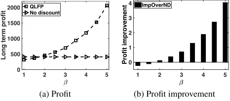
Figure 3 shows the long term profit and the profit im-provement over no discount. Figure 3(a) shows that the long term profit is invariant ofβ when a seller does not provide any discount, while the long term profit under our QLFP algorithm increases significantly in β. Namely, using our QLFP algorithm, the sellers can earn more profit when buy-ers becomes more sensitive to discounts. Observe that when
β is around 1 (i.e., buyers are not sensitive to discounts), our QLFP algorithm has a slightly smaller long term profit than the case of not providing any discount. This uncover a “cost” in inferring buyers’ discount preferences from his-torical transaction data. When buyers are not sensitive to discounts, the cost of inference is larger than the benefit of providing discounts. This “inference cost” exists in general. Figure 3(b) shows that the profit improvement increases in
βand the improvement can be as high as 4 times.
1 2 3 4 5
0 500 1000 1500 2000
Long term profit
QLFP No discount
(a) Profit
1 2 3 4 5 0
1 2 3 4
Profit improvement
ImpOverND
(b) Profit improvement
Figure 3: Impact ofβon profit and ImpOverND.
Lessons learned: Our QLFP algorithm improves the profit over the Q-learning and Speedy Q-learning by as high as 50%, and over the case of not providing any price discount by as high as four times.
Impact of Rating Bias
Now we study the impact of rating bias (i.e., parameter θ
andγ). We fix β = 1and consider the rating bias stated in Eq. (5). Figure 4 and shows the long term profit and the profit improvement. Figure 4(a) and 4(d) show that the long term profit (of QLFP, Q-learning, speedy Q-learning and no discount) is non-decreasing in both θ andγ. This implies that the seller can earn more profit when buyers providing higher ratings. Furthermore, our QLFP has the largest long term profit among these four algorithms. From Figure 4(b) and Figure 4(e) one can observe that the profit improvement is as high as 30% over Q-learning and speedy Q-learning, and as high as two times over the case of no discount. This shows that our QLFP converges faster than Q-learning and speedy Q-learning and effective in inferring the optimal dis-count.
0.2 0.4 0.6 0.8 1
0 100 200 300
Long term profit
QLFP Q-learning Speedy Q-learning No discount =3
(a) Long term profit
0.2 0.4 0.6 0.8 1
0 0.5 1
Profit Improvement
ImpOverQL ImpOverSpeedyQL ImpOverND =3
(b) Profit improvement
1 2 3 4 5
40 60 80 100 120 140
Long term profit
QLFP Q-learning Speedy Q-learning No discount =0.1
(c) Long term profit
0 2 4
0 0.5 1 1.5 2
Profit Improvement
ImpOverQL ImpOverSpeedyQL ImpOverND
=0.1
(d) Profit improvement
Figure 4: Impact of rating bias on profit and ImpOverQL and ImpOverSpeedyQL.
Related Work
From an economic perspective, our work is related to (Landon and Smith 1998; Ba and Pavlou 2002; Jin and Kato 2006). Using a historical transaction dataset from the wine market, Landonet al.(Landon and Smith 1998) uncovered how the reputation of a wine influences its price. In online auction markets, Baet al.(Ba and Pavlou 2002) found that a seller can have some price premiums if she has a high rep-utation, and Jinet al.(Jin and Kato 2006) studied how the reputation influences the pricing behavior of sellers in Inter-net auctions. We study a different problem, i.e., optimizing the reputation & discount trade-offs.
A variety of RL algorithms were designed for SMDP models (Bradtke and Duff 1994), such as the classical Q-learning, temporal difference Q-learning, ATRDP and their variants. We refer the reader to (Bertsekas and Tsitsiklis 1996; Bradtke and Duff 1994; Sutton and Barto 1998) for a thorough treatment on RL. To infer the optimal discount, there are three notable learning like algorithms, i.e., Q-learning (Bradtke and Duff 1994), Speedy Q-Q-learning (Azar et al. 2011), and Zap Q-learning (Devraj and Meyn 2017). Our QLFP algorithm extends the classical Q-learning algo-rithm. We prove the convergence of our QLFP algorithm and show via experiments that our QLFP algorithm improves the profit by as high as 50% over both the classical Q-learning and speedy Q-learning algorithm. We do not compare with the Zap Q-learning algorithm because the it needs to invert a square matrix of order26×106in each iteration, making
it not practical to infer the optimal discount.
Conclusion
This paper develops an online framework to optimize the reputation & discount trade-offs. We formulated a profit maximization problem via an SMDP to explore optimal trade-offs in selecting price discounts. We proved the mono-tonicity of the optimal profit and discount. Based on the monotonicity, we designed a QLFP algorithm, which infers the optimal discount from historical transaction data. We conducted experiments on a dataset from eBay to showed that our QLFP algorithm improves the profit by as high as 50% over the Q-learning and speedy Q-learning algorithm. Our QLFP algorithm also improves the profit by as high as four times over the case of not providing any discount.
Acknowledgments
The work of John C.S. Lui was supported in part by the GRF Funding 14200117. We would like to thank Richard T.B. Ma for his helpful discussions on the paper.
References
Azar, M. G.; Munos, R.; Ghavamzadeh, M.; and Kappen, H. 2011. Speedy q-learning. InAdvances in neural information processing systems.
Ba, S., and Pavlou, P. A. 2002. Evidence of the effect of trust building technology in electronic markets: Price premiums and buyer behavior.MIS quarterly243–268.
Bertsekas, D. P., and Tsitsiklis, J. N. 1996.Neuro-Dynamic Programming. Athena Scientific, 1st edition.
Boyd, S., and Vandenberghe, L. 2004.Convex optimization. Cambridge university press.
Bradtke, S. J., and Duff, M. O. 1994. Reinforcement learn-ing methods for continuous-time markov decision problems. InProc. of NIPS.
Chiang, A. C. 1984. Fundamental methods of mathematical economics.
Dellarocas, C. 2001. Analyzing the economic efficiency of ebay-like online reputation reporting mechanisms. InProc. of ACM EC.
Devraj, A. M., and Meyn, S. 2017. Zap q-learning. In
Advances in Neural Information Processing Systems, 2235– 2244.
eBay. 1995. eBay Classifies Sellers into Twelve Stars. http: //pages.ebay.com/help/feedback/scores-reputation.html. Fortune500. 2015. http://fortune.com/fortune500/.
Jin, G. Z., and Kato, A. 2006. Price, quality, and reputa-tion: Evidence from an online field experiment. The RAND Journal of Economics37(4):983–1005.
Khopkar, T.; Li, X.; and Resnick, P. 2005. Self-selection, slipping, salvaging, slacking, and stoning: The impacts of negative feedback at ebay. InProc. of ACM EC.
Landon, S., and Smith, C. E. 1998. Quality expectations, reputation, and price.Southern Economic Journal628–647. Muchnik, L.; Aral, S.; and Taylor, S. J. 2013. So-cial influence bias: A randomized experiment. Science
341(6146):647–651.
Puterman, M. L. 2014.Markov decision processes: discrete stochastic dynamic programming. John Wiley & Sons. Resnick, P.; Kuwabara, K.; Zeckhauser, R.; and Friedman, E. 2000. Reputation systems. Commun. ACM 43(12):45– 48.
Sutton, R. S., and Barto, A. G. 1998. Reinforcement learn-ing: An introduction, volume 1. MIT press Cambridge. Xie, H., and Lui, J. C. S. 2015. Modeling ebay-like rep-utation systems: Analysis, characterization and insurance mechanism design.Performance Evaluation91:132–149. Xie, H., and Lui, J. C. S. 2017. Mining deficiencies of online reputation systems: Methodologies, experiments and implications.IEEE Transactions on Services Computing. Xie, H.; Li, Y.; and Lui, J. C. 2018. A Reinforce-ment Learning Approach to Optimize Discounts & Reputa-tion Trade-offs in E-commerce Systems.https://1drv.ms/b/s! AkqQNKuLPUbEdgLEiMLJQu8MfZM.
Xie, H.; Ma, R. T. B.; and Lui, J. C. S. 2018. Enhanc-ing reputation via price discounts in e-commerce systems: A data-driven approach. ACM Trans. Knowl. Discov. Data
20(3):26:1–26:29.