The Thirty-Third AAAI Conference on Artificial Intelligence (AAAI-19)
A Comparative Analysis of Expected and Distributional Reinforcement Learning
Clare Lyle,
1Marc G. Bellemare,
2Pablo Samuel Castro
2 1University of Oxford (work done while at Google Brain)2Google Brain
[email protected], [email protected], [email protected]
Abstract
Since their introduction a year ago, distributional approaches to reinforcement learning (distributional RL) have produced strong results relative to the standard approach which models expected values (expected RL). However, aside from con-vergence guarantees, there have been few theoretical results investigating the reasons behind the improvements distribu-tional RL provides. In this paper we begin the investigation into this fundamental question by analyzing the differences in the tabular, linear approximation, and non-linear approx-imation settings. We prove that in many realizations of the tabular and linear approximation settings, distributional RL behaves exactly the same as expected RL. In cases where the two methods behave differently, distributional RL can in fact hurt performance when it does not induce identical behaviour. We then continue with an empirical analysis comparing dis-tributional and expected RL methods in control settings with non-linear approximators to tease apart where the improve-ments from distributional RL methods are coming from.
1
Introduction
The distributional perspective, in which one models the dis-tribution of returns from a state instead of only its expected value, was recently introduced by (Bellemare, Dabney, and Munos 2017). The first distributional reinforcement learning algorithm, C51, saw dramatic improvements in performance in many Atari 2600 games when compared to an algorithm that only modelled expected values (Bellemare, Dabney, and Munos 2017). Since then, additional distributional algorithms have been proposed, such as quantile regression (Dabney et al. 2017) and implicit quantile networks (Dabney et al. 2018), with many of these improving on the results of C51. The abundance of empirical results make it hard to dispute that taking the distributional perspective is helpful in deep rein-forcement learning problems, but theoretical motivation for this perspective is comparatively scarce. Possible reasons for this include the following, proposed by (Bellemare, Dabney, and Munos 2017) .
1. Reduced chattering:modeling a distribution may reduce prediction variance, which may help in policy iteration. 2. Improved optimization behaviour: distributions may
present a more stable learning target, or in some cases Copyright c2019, Association for the Advancement of Artificial Intelligence (www.aaai.org). All rights reserved.
(e.g. the softmax distribution used in the C51 algorithm) have a regularizing effect in optimization for neural net-works.
3. Auxiliary tasks: the distribution offers a richer set of predictions for learning, serving as a set of auxiliary tasks which is tightly coupled to the reward.
Initial efforts to provide a theoretical framework for the anal-ysis of distributional algorithms demonstrated their conver-gence properties (Rowland et al. 2018), and did not directly compare their expected performance to expected algorithms. Indeed, even experimental results supporting the distribu-tional perspective have largely been restricted to the deep reinforcement learning setting, and it is not clear whether the benefits of the distributional perspective also hold in simpler tasks. In this paper we continue lifting the veil on this mystery by investigating the behavioural differences between distri-butional and expected RL, and whether these behavioural differences necessarily result in an advantage for distribu-tional methods.
2
Background
We model the reinforcement learning problem as an agent interacting with an environment so as to maximize cumu-lative discounted reward. We formalize the notion of an environment with a Markov Decision Process (MDP) de-fined as the tuple (X,A, R, P, γ), where X denotes the state space,Athe set of possible actions,R : X × A →
Dist([−RM AX, RM AX]) is a stochastic reward function
mapping state-action pairs to a distribution over a set of bounded rewards,P the transition probability kernel, and
γ∈[0,1)the discount factor.
We denote by π : X → Dist(A) a stochastic policy mapping states to a distribution over actions (i.e.π(a|x)is the agent’s probability of choosing actionain statex). We will use the notationQto refer to state-action value function, which has the typeQ:X × A →R. The value of a specific
policyπis given by the value functionQπ, defined as the
discounted sum of expected future rewards after choosing actionafrom statesand then followingπ
Qπ(x, a) :=Eπ,P
∞
X
t=0
γtR(xt, at)
x0=x, a0=a
One can also express this value as the fixed point of the Bellman operatorTπ(Bellman 1957), defined as
TπQ(x, a) :=E[R(x, a)]
+γX
x0,a0
P(x0|x, a)π(a0|x0)Q(x0, a0).
The Bellman operatorTπdepends on the policyπ, and is used inpolicy evaluation(Sutton and Barto 1998). When we seek to improve the current policy, we enter thecontrol set-ting. In this setting, we modify the previous Bellman operator to obtain the Bellman optimality operatorT∗, given by
T∗Q(x, a) :=E[R(x, a)] +γ X
x0
P(x0|x, a) max a0 Q(x
0, a0).
In many problems of interest, we do not have a full model of the MDP, and instead use a family of stochastic versions of the Bellman operator called temporal difference (TD) up-dates (Sutton and Barto 1998). We will focus on the SARSA update (Rummery and Niranjan 1994), defined as follows. We fix a policy πand let(xt, at, rt, xt+1, at+1)be a
sam-pled transition from the MDP, wherert ∼ R(xt, at) is a
realized reward andat+1 ∼π(·|xt+1). We letαtbe a step
size parameter for timet. Then given a value function esti-mateQt:X × A →Rat timet, the SARSA update gives
the new estimateQt+1:
Qt+1(xt, at) = (1−αt)Qt(xt, at)+αt(rt+γQt(xt+1, at+1)). (1)
Under certain conditions on the MDP andαt, SARSA
con-verges toQπ(Bertsekas 1996).
Semi-gradient SARSA updates extend the SARSA update from the tabular to the function approximation setting. We consider a parameter vectorθt, and feature vectorsφx,afor
each(x, a)∈ X × Asuch that
Qt(x, a) =θTtφx,a.
Givenθt,θt+1is given by thesemigradientupdate (Sutton
and Barto 1998)
θt+1:=θt−αt(θtTφxt,at−rt+γθ
T
tφxt+1,at+1)φxt,at. (2)
Instead of considering only the expected return from a state-action pair, one can consider the distribution of returns. We will use the notation Z : X × A → Dist(R) to de-note areturn distribution function. We can then construct an analogous Bellman operator for these functions, as shown by (Bellemare, Dabney, and Munos 2017) and termed the distributional Bellman operator,Tπ
D:
TDπZ(x, a)=DR(x, a) +γZ(X0, A0) (3) whereX0, A0are the random variables corresponding to the next state and action. This is equality in distribution, and not an equality of random variables.
Analogous to the expected Bellman operator, repeated ap-plication of the distributional Bellman operator can be shown to converge to the true distribution of returns (Bellemare, Dab-ney, and Munos 2017). Later work showed the convergence of stochastic updates in the distributional setting (Rowland et al. 2018). The proof of convergence of the distributional Bellman operator uses a contraction argument, which in the
distributional setting requires us to be careful about how we define the distance between two return distribution functions. Probability divergences and metrics capture this notion of distance. The theoretical properties of some probability distribution metrics have been previously explored by (Gibbs and Su 2002), and the Wasserstein distance in particular studied further in the context of MDPs (Ferns et al. 2012) as well as in the generative model literature (Arjovsky, Chintala, and Bottou 2017). The Wasserstein distance also appears in the distributional reinforcement learning literature, but we omit its definition in favour of the related Cram´er distance, whose properties make it more amenable to the tools we use in our analysis.
The C51 algorithm uses the cross-entropy loss function to achieve promising performance in Atari games; however, the role of the cross-entropy loss in distributional RL has not been the subject of much theoretical analysis. We will use primarily the Cram´er distance (Sz´ekely 2003) in the results that follow, which has been studied in greater depth in the distributional RL literature. Motivations for the use of this distance have been previously outlined for generative models (Bellemare et al. 2017).
Definition 1(Cram´er Distance). LetP, Qbe two probability distributions with Cumulative Distribution Functions (CDFs)
FP, FQ. The Cram´er metric`2betweenP andQis defined
as follows:
`2(P, Q) = s
Z
R
(FP(x)−FQ(x))2dx
We will overload notation and write equivalently`2(P, Q)≡
`2(FP, FQ)or, whenX andY are random variables with
lawsP andQ,`2(P, Q)≡`2(X, Y).
Practically, distributional reinforcement learning algo-rithms require that we approximate distributions. There are many ways one can do this, for example by predict-ing the quantiles of the return distribution (Dabney et al. 2017). In our analysis we will focus on the class of categor-ical distributions with finite support. Given some fixed set
z={z1, . . . , zK} ∈RK withz1≤z2≤ · · · ≤zK, a
cate-gorical distributionP with supportzis a mixture of Dirac measures on each of thezi’s, having the form
P ∈ Zz:=
(K
X
i=1
αiδzi :αi ≥0,
K X
i=1
αi= 1 )
. (4)
Under this class of distributions, the Cram´er distance be-comes a finite sum
`2(FP, FQ) = v u u t
K−1 X
i=1
(zi+1−zi)(FP(zi)−FQ(zi))2
which amounts to a weighted Euclidean norm between the CDFs of the two distributions. When the atoms of the support are equally spaced apart, we get a scalar multiple of the Euclidean distance between the vectors of the CDFs.
Definition 2(Cram´er Projection). Letzbe an ordered set ofK real numbers. For a Dirac measure δy, the Cram´er
projectionΠC(δy)onto the supportzis given by:
ΠC(δy) =
δz1 ify≤z1
zi+1−y
zi+1−ziδzi+
y−zi
zi+1−ziδzi+1 ifzi< y≤zi+1
δzK ify > zK
The operatorΠChas two notable properties: first, as hinted
by the nameCram´er projection, it produces the distribution supported onzwhich minimizes the Cram´er distance to the original distribution. Second, if the support of the distribu-tion is contained in the interval[z1, zK], we can show that
the Cram´er projection preserves the distribution’s expected value 1. It is thus a natural approximation tool for categorical distributions.
Proposition 1. Letz ∈ Rk, andP be a mixture of Dirac
distributions (see Eq. 4) whose support is contained in the interval[z1, zK]. Then the Cram´er projectionΠC(P)ontoz
is such that
E[ΠC(P)] =E[P]
.
The Cram´er projection is implicit in the C51 algorithm, introduced by (Bellemare, Dabney, and Munos 2017). The C51 algorithm uses a deep neural network to compute a softmax distribution, then updates its weights according to the cross-entropy loss between its prediction and a sampled target distribution, which is then projected onto the support of the predicted distribution using the Cram´er projection.
3
The Coupled Updates Method
We are interested in the behavioural differences (or lack thereof) between distributional and expected RL algorithms. We will study these differences through a methodology where we couple the experience used by the update rules of the two algorithms.
Under this methodology, we consider pairs of agents: one that learns a value function (theexpectation learner) and one that learns a value distribution (thedistribution learner). The output of the first learner is a sequence of value functions
Q1, Q2, . . .. The output of the second is a sequence of value
distributionsZ1, Z2, . . .. More precisely, each sequence is
constructed via some update rule:
Qt+1:=UE(Qt, ωt) Zt+1:=UD(Zt, ωt),
from initial conditionsQ0andZ0, respectively, and where
ωtis drawn from some sample spaceΩ. These update rules
may be deterministic (for example, an application of the Bellman operator) or random (a sample-based update such as TD-learning). Importantly, however, the two updates may be coupled through the common sampleωt. Intuitively,Ωcan
be thought of as the source of randomness in the MDP. Key to our analysis is to study update rules that are ana-logues of one another. IfUE is the Bellman operator, for
example, then UD is the distributional Bellman operator.
More generally speaking, we will distinguish between model-basedupdate rules, which do not depend onωt, and
sample-based update rules, which do. In the latter case, we will
assume access to a scheme that generates sample transi-tions based on the sequence ω1, ω2, . . ., that is, a
genera-tor G : ω1, . . . , ωt 7→ (xt, at, rt, xt+1, at+1). Under this
scheme, a pair UE, UD of sampled-based update rules
re-ceive exactly the same sample transitions (for each possible realization); hence thecoupled updates method, inspired by the notion of coupling from the probability theory literature (Thorisson 2000).
The main question we will answer is: which analogue update rules preserve expectations?Specifically, we write
Z =E Q ⇐⇒ E[Z(x, a)] =Q(x, a) ∀(x, a)∈ X × A.
We will say that analogue rulesUDandUEare
expectation-equivalentif, for all sequences(ωt), and for allZ0andQ0,
Z0=E Q0 ⇐⇒ Zt=E Qt ∀t∈N.
Our coupling-inspired methodology will allow us to rule out a number of common hypotheses regarding the good performance of distributional reinforcement learning:
Distributional RL reduces variance.By our coupling argu-ment, any expectation-equivalent rulesUDandUEproduce
exactly the same sequence of expected values,along each sample trajectory. The distributions of expectations relative to the random drawsω1, ω2, . . . are identical and therefore,
Var[EZt(x, a)] = Var[Qt(x, a)]everywhere, andUD does
not produce lower variance estimates.
Distributional RL helps with policy iteration.One may imagine that distributional RL helps identify the best action. But ifZt=E Qteverywhere, then also greedy policies based
onarg maxQt(x,·)andarg maxEZt(x,·)agree. Hence our
results (presented in the context of policy evaluation) extend to the setting in which actions are selected on the basis of their expectation (e.g.-greedy, softmax).
Distributional RL is more stable with function approxi-mation.We will use the coupling methodology to provide evidence that, at least combined with linear function approx-imation, distributional update rules do not improve perfor-mance.
4
Analysis of Behavioural Differences
Our coupling-inspired methodology provides us with a sta-ble framework to perform a theoretical investigation of the behavioural differences between distributional and expected RL. We use it through a progression of settings that will gradually increase in complexity to shed light on what causes distributional algorithms to behave differently from expected algorithms. We consider three axes of complexity: 1) how we approximate the state space, 2) how we represent the dis-tribution, and 3) how we perform updates on the predicted distribution function.4.1
Tabular models
functions andQfor the space of bounded value functions. We begin with results regarding two model-based update rules.
Proposition 2. LetZ0∈ ZandQ0∈ Q, and suppose that
Z0=E Q0. If
Zt+1:=TDπZt Qt+1:=TπQt,
then alsoZt=E Qt∀t∈N.
See the supplemental material for the proof of this result and those that follow.
We next consider a categorical, tabular representation where the distribution at each state-action pair is stored ex-plicitly but, as per Equation (4), restricted to the finite support
z={z1, . . . , zK}, (Rowland et al. 2018). Unlike the tabular
representation of Prop. 2, this algorithm has a practical im-plementation; however, after each Bellman update we must project back the result into the space of those finite-support distributions, giving rise to a projected operator.
Proposition 3. Suppose that the finite support brackets the set of attainable value distributions, in the sense thatz1≤
−RMAX
1−γ andzK ≥ RMAX
1−γ. Define the projected distributional
operator
TCπ:= ΠCTDπ. SupposeZ0=E Q0, forZ0∈ Zz, Q0∈ Q. If
Zt+1:=TCπZt Qt+1:=TπQt,
then alsoZt=E Qt∀t∈N.
Next, we consider sample-based update rules, still in the tabular setting. These roughly correspond to the Categori-cal SARSA algorithm whose convergence was established by (Rowland et al. 2018), with or without the projection step. Here we highlight the expectation-equivalence of this algorithm to the classic SARSA algorithm (Rummery and Niranjan 1994).
For these results we will need some additional notation. Consider a sample transition(xt, at, rt, xt+1, at+1). Given a
random variableY, denote its probability distribution byPY
and its cumulative distribution function byFY, respectively.
With some abuse of notation we extend this to value distribu-tions and writePZ(x, a)andFZ(x, a)for the probability
dis-tribution and cumulative disdis-tribution function, respectively, corresponding toZ(x, a). Finally, letZt0(xt, at)be a random
variable distributed like the targetrt+γZt(xt+1, at+1), and
writeΠCZt0(x, a)for its Cram´er projection onto the support z.
Proposition 4. Suppose thatZ0 ∈ Z, Q0 ∈ QandZ0 =E
Q0. Given a sample transition(xt, at, rt, xt+1, at+1)
con-sider the mixture update
PZt+1(x, a) :=
(1−αt)PZt(x, a) +αtPZ0t(xt, at)
PZt(x, a) ifx, a6=xt, at and the SARSA update
Qt+1(xt, at) :=
Qt(xt, at) +αtδt
Qt(x, a) ifx, a6=xt, at
whereδt:= (rt+γQt(xt+1, at+1)−Qt(xt, at)), then also
Zt=E Qt∀t∈N.
Proposition 5. Suppose thatZ0 ∈ Zz, Q0 ∈ Q,Z0 =E Q0,
thatzbrackets the set of attainable value distributions, and
PZ0
t in Prop. 4 is replaced by the projected targetPΠCZt0. Then alsoZt=E Qt∀t∈N.
Together, the propositions above show that there is no benefit, at least in terms of modelling expectations, to using distributional RL in a tabular setting when considering the distributional analogues of update rules in common usage in reinforcement learning.
Next we turn our attention to a slightly more complex case, where distributional updates correspond to a semi-gradient update. In the expected setting, the mixture update of Prop. 4 corresponds to taking the semi-gradient of the squared loss of the temporal difference errorδt. While there is no simple
no-tion of semi-gradient whenZis allowed to represent arbitrary distributions inZ, there is when we consider a categorical representation, which is a finite object whenX andAare finite (specifically,Z can be represented by|X ||A|Kreal values).
To keep the exposition simple, in what follows we ignore the fact that semi-gradient updates may yield an object which is not a probability distribution proper. In particular, the argu-ments remain unchanged if we allow the learner to output a signed distribution, as argued by (Bellemare et al. 2019).
Definition 3(Gradient of Cram´er Distance). LetZ, Z0∈ Zz
be two categorical distributions supported onz. We define the gradient of the squared Cram´er distance with respect to the CDF ofZ, denoted∇F`22(Z, Z0)∈RKas follows:
∇F`22(Z, Z0)[i] :=
∂ ∂F(zi)
`22(Z, Z0).
Similarly,
∇P`22(Z, Z0)[i] :=
∂ ∂P(zi)
`22(Z, Z0).
We say that the categorical supportzisc-spacedifzi+1−
zi=cfor alli(recall thatzi+1≥zi).
Proposition 6. Suppose that the categorical supportzisc -spaced. LetZ0∈ Z, Q0∈ Qbe such thatZ0=E Q0. Suppose
thatQt+1is updated according to the SARSA update with
step-sizeαt. LetZt0be given byΠC(rt+γZt(xt+1, at+1)).
Consider the CDF gradient update rule
FZt+1(x, a) :=
FZt(x, a) +α
0
t∇F`22(Zt(xt, at), Zt0(xt, at))
FZt(x, a) ifx, a6=xt, at.
Ifα0
t= αt
2c, then alsoZt E
=Qt∀t∈N.
Proposition 7. Suppose the CDF gradient in update rule of Prop. 6 is replaced by the PDF gradient∇P`22(Zt, Zt0). Then
for each choice of step-sizeα0there exists an MDPM and a time stept∈Nfor whichZ0=E Q0butZt
E
6
=Qt.
The counterexample used in the proof of Prop. 7 illustrates what happens when the gradient is taken w.r.t. the probability mass: some atoms of the distribution may be assigned nega-tive probabilities. Including a projection step does not rectify the issue, as the expectation ofZtremains different fromQt.
4.2
Linear Function Approximation
In the linear approximation setting, we represent each state-action pairx, aas afeature vectorφx,a ∈Rd, We wish to
find a linear function given by a weight vectorθsuch that
θTφx,a≈Qπ(x, a).
In the categorical distributional setting,θbecomes a matrix
W ∈RK×d. Here we will consider approximating the
cumu-lative distribution function:
FZ(x,a)(zi) =W φx,a[i].
We can extend this parametric form by viewingF as de-scribing the CDF of a mixture of Diracs (Equation 4). Thus,
F(z) = 0 forz < z1, and similarly F(z) = F(zk)for
z≥zk; see (Bellemare et al. 2019) for a justification. In what
follows we further assume that the supportzis1-spaced. In this setting, there may be noWfor whichFZ(x, a)
de-scribes a proper cumulative distribution function: e.g.F(y)
may be less than or greater than 1 fory > zk. Yet, as shown
by (Bellemare et al. 2019), we can still analyze the behaviour of a distributional algorithm which is allowed to output im-proper distributions. In our analysis we will assume that all predicted distributions sum to 1, though they may assign negative mass to some outcomes.
We writeQφ := {θ>φ : θ ∈ Rd} for the set of value
functions that can be represented by a linear approximation overφ. Similarly,Zφ :={W φ:W ∈RK×d}is the set of
CDFs that are linearly representable. ForZt ∈ Zφ, letWt
be the corresponding weight matrix. As before, we define
Zt0(xt, at)to be the random variable corresponding to the
projected targetΠC[rt+γZt(xt+1, at+1)].
Proposition 8. Let Z0 ∈ Zφ,Q0 ∈ Qφ, andz ∈ RK
such thatzis 1-spaced. Suppose thatZ0 =E Q0, and that
Z0(x, a)[zK] = 1∀x, a. LetWt, θtrespectively denote the
weights corresponding toZtandQt. IfZt+1 is computed
from the semi-gradient update rule
Wt+1:=Wt+αt(FZ0
t(xt, at)−Wtφxt,at)φ
T xt,at
andQt+1is computed according to Equation 2 with the same
step-sizeαt, then alsoZt=E Qt∀t∈N.
Importantly, the gradient in the previous proposition is taken with respect to the CDF of the distribution. Taking the gradient with respect to the Probability Mass Function (PMF) does not preserve the expected value of the predictions, which we have already shown in the tabular setting. This negative result is consistent with the results on signed distributions by (Bellemare et al. 2019).
4.3
Non-linear Function Approximation
To conclude this theoretical analysis, we consider more gen-eral function approximation schemes, which we will refer to as the non-linear setting. In the non-linear setting, we consider a differentiable functionψ(W,·). For example, the functionψ(W, φx,a)could be a probability mass function
given by a softmax distribution over the logitsW φx,a, as is
the case for the final layer of the neural network in the C51 algorithm.
Proposition 9. There exists a (nonlinear) representation of the cumulative distribution function parametrized by
W ∈RK×dsuch thatZ
0=E Q0but after applying the
semi-gradient update rule
Wt+1:=Wt+αt∇W`22(ψ(W, φ(xt, at)), FZ0
t), whereFZ0
tis the cumulative distribution function of the
pro-jected Bellman target, we haveZ1 E
6
=Q1.
The key difference with Prop. 8 is the change from the gradient of a linear function (the feature vectorφxt,at) to the
gradient of a nonlinear function; hence the result is not as trivial as it might look. Still, while the result is not altogether surprising, combined with our results in the linear case it shows that the interplay with nonlinear function approxima-tion is a viable candidate for explaining the benefits of the distributional approach. In the next section we will present empirical evidence to this effect.
5
Empirical Analysis
Our theoretical results demonstrating that distributional RL often performs identically to expected RL contrast with the empirical results of (Bellemare, Dabney, and Munos 2017; Dabney et al. 2017; 2018; Barth-Maron et al. 2018; Hes-sel et al. 2018), to name a few. In this section we confirm our theoretical findings by providing empirical evidence that distributional reinforcement learning does not improve perfor-mance when combined with tabular representations or linear function approximation. Then, we find evidence of improved performance when combined with deep networks, suggesting that the answer lies, as suggested by Prop. 9, in distributional reinforcement learning’s interaction with nonlinear function approximation.
5.1
Tabular models
Figure 1: Cartpole (left) and Acrobot (right) with Fourier features of order 4. Step size in parentheses. Algorithms correspond to the lite versions described in text.
Figure 2: Varying the basis orders on CartPole. Orders 1 (left), 2 (center), 3 (right). Step sizes same as in Fig.1.
not significantly worse in performance, did exhibitdifferent
performance, performing better on some random seeds and worse on others than expected Q-learning. We observed a similar phenomenon with a simple 3-state chain MDP. Re-sults for both experiments are omitted for brevity, but are included in the supplemental material.
5.2
Linear Function Approximation
We next investigate whether the improved performance of distributional RL is due to the outputs and loss functions used, and whether this can be observed even with linear function approximation.
We make use of three variants of established algorithms for our investigation, modified to use linear function approxi-mators rather than deep networks. We include in this analysis an algorithm that computes a softmax over logits that are a linear function of a state feature vector. Although we did not include this type of approximator in the linear setting of our theoretical analysis, we include it here as it provides an analogue of C51 against which we can compare the other algorithms.
1. DQN-lite, based on (Mnih et al. 2015), predictsQ(x, a), the loss is the squared difference between the target and the prediction.
2. C51-lite, based on (Bellemare, Dabney, and Munos 2017), outputsZ(x, a), a softmax distribution whose logits are
linear inφx,a. It minimizes the cross-entropy loss between
the target and the prediction.
3. S51-lite, based on (Bellemare et al. 2019), outputsZ(x, a)
as a categorical distribution whose probabilities are a linear function of φx,a and minimizes the squared
Cram´er distance.
We further break S51-lite down into two sub-methods. One of these performs updates by taking the gradient of the Cram´er distance with respect to the points of the PMF of the prediction, while the other takes the gradient with respect to the CDF. For a fair comparison, all algorithms used a stochastic gradient descent optimizer except where noted. We used the same hyperparameters for all algorithms, except for step sizes, where we chose the step size that gave the best performance for each algorithm. We otherwise use the usual agent infrastructure from DQN, including a replay memory of capacity 50,000 and a target network which is updated after every 10 training steps. We update the agent by sampling batches of 128 transitions from the replay memory.
We ran these algorithms on two classic control environ-ments: CartPole and Acrobot. In CartPole, the objective is to keep a pole balanced on a cart by moving the cart left and right. In Acrobot, the objective is to swing a double-linked pendulum above a threshold by applying torque to one of its joints. We encode each original statex, (x∈R4for CartPole
andx∈R6for Acrobot) as a feature vectorφ(x)given by
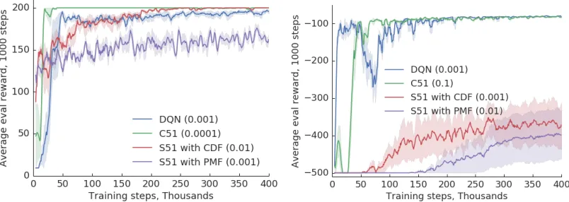
Figure 3: Cartpole with Adam optimizer (left) and Acrobot (right) with deep networks. Learning rate parameter in parentheses.
and Thomas 2011). For completeness, on Cartpole the basis of order 1 yields 15 features, order 2: 80 features, 3: 255, and finally 4: 624 features.
We first compare how DQN-, C51-, and S51-lite perform on the two tasks in Figure 1 with the order 4 basis, which is more than sufficient to well-approximate the value function. We observe that DQN learns more quickly than C51 and S51 with CDF, while S51 with PMF underperforms signifi-cantly. On Acrobot, the difference is even more pronounced. This result at first glance seems to contradict the theoretical result we showed indicating that S51-lite should perform similarly to DQN in the linear function approximation case, but we attribute this difference in performance to the fact that the initialization in the S51 algorithm doesn’t enforce the assumption that the predicted distributions sum to 1.
We then investigate the effect of reducing the order in all algorithms in Figure 2. We observe that the distributional algorithms performs poorly when there are too few features; by contrast, DQN-lite can perform both tasks with an order 2 basis. This indicates that the distributional methods suffered more when there were fewer informative features available than expectation-based methods did in this setting.
5.3
Nonlinear function approximation
We repeat the above experiment, but now replace the Fourier basis features with a two-layer ReLU neural network that is trained along with the final layer (which remains linear). In the CartPole task we found that DQN often diverged with the gradient descent optimizer, so we used Adam for all the algorithms, and chose the learning rate parameter that gave the best performance for each. Results are displayed in Figure 3. We can observe that C51 generally outperforms DQN, although they both eventually converge to the same value. It is interesting to notice that S51 has a harder time achieving the same performance, and comes nowhere near in the harder Acrobot task. This suggests that despite being theoretically unnecessary, the softmax in C51 is working to its advantage. This finding is consistent with the empirical results observed in Atari games by (Bellemare et al. 2019).
The results of the previous two sets of experiments indicate that the benefits of distributional reinforcement learning are
primarily gained from improved learning in the earlier layers of deep neural networks, as well as in the nonlinear softmax used in C51. We believe further investigations in this direction should lead to a deeper understanding of the distributional approach.
6
Discussion and Future Work
In this paper we have provided theoretical and empirical results that give evidence on the benefits (or, some cases, lack thereof) of the distributional approach in reinforcement learning. Together, our results point to function approxima-tion as the key driver in the difference in behaviour between distributional and expected algorithms.
To summarize, our findings are:
1. Distributional methods are generally expectation-equivalent when using tabular representations or linear function approximation, but
2. diverge from expected methods when we use non-linear function approximation.
3. Empirically, we provide fresh confirmation that modelling a distribution helps when using non-linear approximation. There are a few notions from distributional reinforcement learning not covered by our study here, including the effect of using Wasserstein projections of the kind implied by quantile regression (Dabney et al. 2017), and the impact of the softmax transfer function used by C51 on learning. In particular the regression setting, (Imani and White 2018) show that even for a fixed set of features, optimizing a distributional loss results in better accuracy than minimizing the squared error of predictions.
Yet we believe the most important question raised by our work is: what happens in deep neural networks that benefits most from the distributional perspective? Returning to the proposed reasons for the distributional perspective’s success in the introduction, we note that the potentially regularizing effect of modeling a distribution, and a potential role as an ‘auxiliary task’ played by the distribution are both avenues
References
Arjovsky, M.; Chintala, S.; and Bottou, L. 2017. Wasserstein generative adversarial networks. InProceedings of the 34th International Conference on Machine Learning, volume 70 ofProceedings of Machine Learning Research, 214–223. International Convention Centre, Sydney, Australia: PMLR. Barth-Maron, G.; Hoffman, M. W.; Budden, D.; Dabney, W.; Horgan, D.; TB, D.; Muldal, A.; Heess, N.; and Lillicrap, T. 2018. Distributional policy gradients. InProceedings of the International Conference on Learning Representations, to appear.
Bellemare, M. G.; Danihelka, I.; Dabney, W.; Mohamed, S.; Lakshminarayanan, B.; Hoyer, S.; and Munos, R. 2017. The cramer distance as a solution to biased wasserstein gradients.
CoRRabs/1705.10743.
Bellemare, M. G.; Roux, N. L.; Castro, P. S.; and Moitra., S. 2019. Distributional reinforcement learning with linear func-tion approximafunc-tion.To appear in Proceedings of AISTATS. Bellemare, M. G.; Dabney, W.; and Munos, R. 2017. A distri-butional perspective on reinforcement learning. In Precup, D., and Teh, Y. W., eds.,Proceedings of the 34th International Conference on Machine Learning, volume 70 of Proceed-ings of Machine Learning Research, 449–458. International Convention Centre, Sydney, Australia: PMLR.
Bellman. 1957. Dyamic programming.
Bertsekas, I. 1996. Temporal differences-based policy itera-tion and applicaitera-tions in neuro-dynamic programming. Dabney, W.; Rowland, M.; Bellemare, M. G.; and Munos, R. 2017. Distributional reinforcement learning with quantile regression.CoRRabs/1710.10044.
Dabney, W.; Ostrovski, G.; Silver, D.; and Munos, R. 2018. Implicit quantile networks for distributional reinforcement learning. 80:1096–1105.
Ferns, N.; Castro, P. S.; Precup, D.; and Panangaden, P. 2012. Methods for computing state similarity in markov decision processes.CoRRabs/1206.6836.
Gibbs, A., and Su, F. 2002. On Choosing and Bounding Probability Metrics. International Statistical Review30:419– 435.
Hessel, M.; Modayil, J.; van Hasselt, H.; Schaul, T.; Ostro-vski, G.; Dabney, W.; Horgan, D.; Piot, B.; Azar, M.; and Silver, D. 2018. Rainbow: Combining improvements in deep reinforcement learning. InProceedings of the AAAI Conference on Artificial Intelligence.
Imani, E., and White, M. 2018. Improving regression perfor-mance with distributional losses. 80.
Konidaris, G.; Osentoski, S.; and Thomas, P. S. 2011. Value function approximation in reinforcement learning using the fourier basis. InProceedings of the AAAI Conference. Mnih, V.; Kavukcuoglu, K.; Silver, D.; Rusu, A. A.; Veness, J.; Bellemare, M. G.; Graves, A.; Riedmiller, M.; Fidjeland, A. K.; Ostrovski, G.; Petersen, S.; Beattie, C.; Sadik, A.; Antonoglou, I.; King, H.; Kumaran, D.; Wierstra, D.; Legg, S.; and Hassabis, D. 2015. Human-level control through deep reinforcement learning. Nature518(7540):529–533.
Rowland, M.; Bellemare, M.; Dabney, W.; Munos, R.; and Teh, Y. W. 2018. An analysis of categorical distributional reinforcement learning. In Storkey, A., and Perez-Cruz, F., eds.,Proceedings of the Twenty-First International Confer-ence on Artificial IntelligConfer-ence and Statistics, volume 84 of
Proceedings of Machine Learning Research, 29–37. Playa Blanca, Lanzarote, Canary Islands: PMLR.
Rummery, G. A., and Niranjan, M. 1994. On-line Q-learning using connectionist systems. Technical report, Cambridge University Engineering Department.
Sutton, R. S., and Barto, A. G. 1998. Introduction to Rein-forcement Learning. Cambridge, MA, USA: MIT Press, 1st edition.