The Thirty-Third AAAI Conference on Artificial Intelligence (AAAI-19)
Bayesian Graph Convolutional Neural
Networks for Semi-Supervised Classification
Yingxue Zhang
∗ Huawei Noah’s Ark Lab Montreal Research Centre 7101 Avenue du Parc, H3N 1X9Montreal, QC Canada
Soumyasundar Pal,
∗Mark Coates
Dept. Electrical and Computer EngineeringMcGill University 3480 University St, H3A 0E9
Montreal, QC, Canada
Deniz ¨
Ustebay
Huawei Noah’s Ark Lab Montreal Research Centre 7101 Avenue du Parc, H3N 1X9Montreal, QC Canada
Abstract
Recently, techniques for applying convolutional neural net-works to graph-structured data have emerged. Graph con-volutional neural networks (GCNNs) have been used to ad-dress node and graph classification and matrix completion. Although the performance has been impressive, the current implementations have limited capability to incorporate un-certainty in the graph structure. Almost all GCNNs process a graph as though it is a ground-truth depiction of the re-lationship between nodes, but often the graphs employed in applications are themselves derived from noisy data or mod-elling assumptions. Spurious edges may be included; other edges may be missing between nodes that have very strong relationships. In this paper we adopt a Bayesian approach, viewing the observed graph as a realization from a paramet-ric family of random graphs. We then target inference of the joint posterior of the random graph parameters and the node (or graph) labels. We present the Bayesian GCNN framework and develop an iterative learning procedure for the case of assortative mixed-membership stochastic block models. We present the results of experiments that demonstrate that the Bayesian formulation can provide better performance when there are very few labels available during the training pro-cess.
1
Introduction
Novel approaches for applying convolutional neural net-works to graph-structured data have emerged in recent years. Commencing with the work in (Bruna et al. 2013; Henaff, Bruna, and LeCun 2015), there have been numer-ous developments and improvements. Although these graph convolutional neural networks (GCNNs) are promising, the current implementations have limited capability to handle uncertainty in the graph structure, and treat the graph topol-ogy as ground-truth information. This in turn leads to an in-ability to adequately characterize the uncertainty in the pre-dictions made by the neural network.
In contrast to this past work, we employ a Bayesian framework and view the observed graph as a realization from a parametric random graph family. The observed ad-jacency matrix is then used in conjunction with features and labels to perform joint inference. The results reported in this
∗
These authors contributed equally to this work.
Copyright c2019, Association for the Advancement of Artificial Intelligence (www.aaai.org). All rights reserved.
paper suggest that this formulation, although computation-ally more demanding, can lead to an ability to learn more from less data, a better capacity to represent uncertainty, and better robustness and resilience to noise or adversarial attacks.
In this paper, we present the novel Bayesian GCNN framework and discuss how inference can be performed. To provide a concrete example of the approach, we focus on a specific random graph model, the assortative mixed mem-bership block model. We address the task of semi-supervised classification of nodes and examine the resilience of the derived architecture to random perturbations of the graph topology.
2
Related work
A significant body of research focuses on using neural net-works to analyze structured data when there is an underlying graph describing the relationship between data items. Early work led to the development of the graph neural network (GNN)(Frasconi, Gori, and Sperduti 1998; Scarselli, Gori, and others 2009; Li et al. 2016b). The GNN approaches rely on recursive processing and propagation of informa-tion across the graph. Training can often take a long time to converge and the required time scales undesirably with re-spect to the number of nodes in the graph, although recently an approach to mitigate this has been proposed by (Liao, Brockschmidt, and others 2018).
Graph convolutional neural networks (GCNNs) have emerged more recently, with the first proposals in (Bruna et al. 2013; Henaff, Bruna, and LeCun 2015; Duvenaud, Maclaurin, and others 2015). A spectral filtering approach was introduced in (Defferrard, Bresson, and Vandergheynst 2016) and this method was simplified or improved in (Kipf and Welling 2017; Levie, Monti, and others 2017; Chen, Ma, and Xiao 2018). Spatial filtering or aggregation strate-gies were adopted in (Atwood and Towsley 2016; Hamilton, Ying, and Leskovec 2017). A general framework for train-ing neural networks on graphs and manifolds was presented by (Monti, Boscaini, and others 2017) and the authors ex-plain how several of the other methods can be interpreted as special cases.
have also demonstrated that gates, edge conditioning, and skip connections can prove beneficial (Bresson and Laurent 2017; Sukhbaatar, Szlam, and Fergus 2016; Simonovsky and Komodakis 2017). In some problem settings it is also bene-ficial to consider an ensemble of graphs (Anirudh and Thia-garajan 2017), multiple adjacency matrices (Such, Sah, and others 2017) or the dual graph (Monti, Shchur, and others 2018). Compared to this past work, the primary methodolog-ical novelty in our proposed approach involves the adoption of a Bayesian framework and the treatment of the observed graph as additional data to be used during inference.
There is a rich literature on Bayesian neural networks, commencing with pioneering work (Tishby, Levin, and Solla 1989; Denker and Lecun 1991; MacKay 1992; Neal 1993) and extending to more recent contributions (Hern´andez-Lobato and Adams 2015; Gal and Ghahramani 2016; Sun, Chen, and Carin 2017; Louizos and Welling 2017). To the best of our knowledge, Bayesian neural networks have not yet been developed for the analysis of data on graphs.
3
Background
Graph convolutional neural networks (GCNNs)
Although graph convolutional neural networks can be ap-plied to a variety of inference tasks, in order to make the description more concrete we consider the task of identify-ing the labels of nodes in a graph. Suppose that we observe a graphGobs= (V,E), comprised of a set ofNnodesVand aset of edgesE. For each node we measure data (or derive fea-tures), denotedxifor nodei. For some subset of the nodes
L ⊂ V, we can also measure labelsYL = {yi : i ∈ L}.
In a classification context, the labelyiidentifies a category;
in a regression contextyican be real-valued. Our task is to
use the featuresxand the observed graph structureGobsto
estimate the labels of the unlabelled nodes.
A GCNN performs this task by performing graph convo-lution operations within a neural network architecture. Col-lecting the feature vectors as the rows of a matrixX, the layers of a GCNN (Defferrard, Bresson, and Vandergheynst 2016; Kipf and Welling 2017) are of the form:
H(1) =σ(AGXW(0)) (1)
H(l+1)=σ(AGH(l)W(l)) (2)
Here W(l) are the weights of the neural network at layer l,H(l) are the output features from layer l−1, and σ is a non-linear activation function. The matrixAG is derived from the observed graph and determines how the output features are mixed across the graph at each layer. The fi-nal output for anL-layer network isZ = H(L). Training
of the weights of the neural network is performed by back-propagation with the goal of minimizing an error metric be-tween the observed labels Y and the network predictions
Z. Performance improvements can be achieved by enhanc-ing the architecture with components that have proved useful for standard CNNs, including attention nodes (Veliˇckovi´c et al. 2018), and skip connections and gates (Li et al. 2016b; Bresson and Laurent 2017).
Although there are many different flavours of GCNNs, all current versions process the graph as though it is a ground-truth depiction of the relationship between nodes. This is despite the fact that in many cases the graphs employed in applications are themselves derived from noisy data or modelling assumptions. Spurious edges may be included; other edges may be missing between nodes that have very strong relationships. Incorporating attention mechanisms as in (Veliˇckovi´c et al. 2018) addresses this to some extent; at-tention nodes can learn that some edges are not represen-tative of a meaningful relationship and reduce the impact that the nodes have on one another. But the attention mecha-nisms, for computational expediency, are limited to process-ing existprocess-ing edges — they cannot create an edge where one should probably exist. This is also a limitation of the en-semble approach of (Anirudh and Thiagarajan 2017), where learning is performed on multiple graphs derived by erasing some edges in the graph.
Bayesian neural networks
We consider the case where we have training inputsX =
{x1, ..., xn} and corresponding outputsY = {y1, ..., yn}.
Our goal is to learn a function y = f(x)via a neural net-work with fixed configuration (number of layers, activation function, etc., so that the weights are sufficient statistics for f) that provides a likely explanation for the relationship be-tweenxandy. The weightsW are modelled as random vari-ables in a Bayesian approach and we introduce a prior dis-tribution over them. SinceWis not deterministic, the output of the neural network is also a random variable. Prediction for a new inputxcan be formed by integrating with respect to the posterior distribution ofW as follows:
p(y|x,X,Y) =
Z
p(y|x, W)p(W|X,Y)dW . (3)
The termp(y|x, W)can be viewed as a likelihood; in a clas-sification task it is modelled using a categorical distribution by applying a softmax function to the output of the neural network; in a regression task a Gaussian likelihood is often an appropriate choice. The integral in eq. (3) is in general intractable. Various techniques for inference ofp(W|X,Y)
have been proposed in the literature, including expectation propagation (Hern´andez-Lobato and Adams 2015), varia-tional inference (Gal and Ghahramani 2016; Sun, Chen, and Carin 2017; Louizos and Welling 2017), and Markov Chain Monte Carlo methods (Neal 1993; Korattikara et al. 2015; Li et al. 2016a). In particular, in (Gal and Ghahramani 2016), it was shown that with suitable variational approximation for the posterior ofW, Monte Carlo dropout is equivalent to drawing samples ofW from the approximate posterior and eq. (3) can be approximated by a Monte Carlo integral as follows:
p(y|x,X,Y)≈ 1 T
S X i=1
p(y|x, Wi), (4)
4
Methodology
We consider a Bayesian approach, viewing the observed graph as a realization from a parametric family of random graphs. We then target inference of the joint posterior of the random graph parameters, weights in the GCNN and the node (or graph) labels. Since we are usually not directly interested in inferring the graph parameters, posterior esti-mates of the labels are obtained by marginalization. The goal is to compute the posterior probability of labels, which can be written as:
p(Z|YL,X,Gobs) = Z
p(Z|W,G,X)p(W|YL,X,G)
p(G|λ)p(λ|Gobs)dW dGdλ . (5)
HereW is a random variable representing the weights of a Bayesian GCNN over graphG, andλdenotes the parame-ters that characterize a family of random graphs. The term p(Z|W,G,X) can be modelled using a categorical distri-bution by applying a softmax function to the output of the GCNN, as discussed above.
This integral in eq. (5) is intractable. We can adopt a number of strategies to approximate it, including variational methods and Markov Chain Monte Carlo (MCMC). For example, in order to approximate the posterior of weights p(W|YL,X,G), we could use variational inference (Gal and Ghahramani 2016; Sun, Chen, and Carin 2017; Louizos and Welling 2017) or MCMC (Neal 1993; Korattikara et al. 2015; Li et al. 2016a). Various parametric random graph generation models can be used to modelp(λ|Gobs), for
ex-ample a stochastic block model (Peixoto 2017), a mixed membership stochastic block model (Airoldi et al. 2009), or a degree corrected block model (Peng and Carvalho 2016). For inference of p(λ|Gobs), we can use MCMC (Li, Ahn,
and Welling 2016) or variational inference (Gopalan, Ger-rish, and others 2012).
A Monte Carlo approximation of eq. (5) is:
p(Z|YL,X,Gobs)≈
1
V
V X
v
1
NGS NG
X i=1
S X s=1
p(Z|Ws,i,v,Gi,v,X). (6)
In this approximation, V samples λv are drawn from
p(λ|Gobs); the precise method for generating these samples
from the posterior varies depending on the nature of the graph model. TheNGgraphsGi,vare sampled fromp(G|λv)
using the adopted random graph model. S weight matri-ces Ws,i,v are sampled from p(W|YL,X,Gi,v) from the
Bayesian GCN corresponding to the graphGi,v.
Example: Assortative mixed membership
stochastic block model
For the Bayesian GCNNs derived in this paper, we use an assortative mixed membership stochastic block model (a-MMSBM) for the graph (Gopalan, Gerrish, and others 2012; Li, Ahn, and Welling 2016) and learn its parametersλ =
{π, β} using a stochastic optimization approach. The as-sortative MMSBM, described in the following section, is a
good choice to model a graph that has relatively strong com-munity structure (such as the citation networks we study in the experiments section). It generalizes the stochastic block model by allowing nodes to belong to more than one com-munity and to exhibit assortative behaviour, in the sense that a node can be connected to one neighbour because of a re-lationship through community A and to another neighbour because of a relationship through community B.
Since Gobs is often noisy and may not fit the adopted
parametric block model well, sampling πv and βv from
p(π, β|Gobs)can lead to high variance. This can lead to the
sampled graphsGi,vbeing very different fromGobs. Instead,
we replace the integration overπandβwith a maximum a posteriori estimate (MacKay 1996). We approximately com-pute
{π,ˆ βˆ}= arg max
β,π p(β, π|Gobs) (7)
by incorporating suitable priors over β andπand use the approximation:
p(Z|YL,X,Gobs)≈
1
NGS NG
X i=1
S X s=1
p(Z|Ws,i,Gi,X). (8)
In this approximation, Ws,i are approximately sampled
fromp(W|YL,X,Gi)using Monte Carlo dropout over the
Bayesian GCNN corresponding toGi. TheGi are sampled
fromp(G|π,ˆ βˆ).
Posterior inference for the MMSBM
For the undirected observed graphGobs = {yab ∈ {0,1} :
1 ≤ a < b ≤ N}, yab = 0 or 1 indicates absence or
presence of a link between nodeaand nodeb. In MMSBM, each nodeahas aKdimensional community membership probability distribution πa = [πa1, ...πaK]T, where K is
the number of categories/communities of the nodes. For any two nodesaandb, if both of them belong to the same community, then the probability of a link between them is significantly higher than the case where the two nodes belong to different communities (Airoldi et al. 2009). The generative model is described as:
For any two nodesaandb, • Samplezab∼πaandzba∼πb.
• Ifzab = zba = k, sample a linkyab ∼ Bernoulli(βk).
Otherwise,yab∼Bernoulli(δ).
Here,0 ≤ βk ≤ 1is termed community strength of the
k-th community andδ is the cross community link proba-bility, usually set to a small value. The joint posterior of the parametersπandβis given as:
p(π, β|Gobs)∝p(β)p(π)p(Gobs|π, β)
= K
Y
k=1 p(βk)
N
Y
a=1 p(πa)
Y
1≤a<b≤N
X
zab,zba
p(yab, zab, zba|πa, πb, β).
(9)
We use a Beta(η)distribution for the prior ofβk and a
Dirichlet distribution, Dir(α), for the prior of πa, whereη
Expanded mean parameterisation
Maximizing the posterior of eq. (9) is a constrained
opti-mization problem withβk, πak ∈ (0,1)and K X k=1
πak = 1.
Employing a standard iterative algorithm with a gradient based update rule does not guarantee that the constraints will be satisfied. Hence we consider an expanded mean pa-rameterisation (Patterson and Teh 2013) as follows. We in-troduce the alternative parametersθk0, θk1 ≥ 0 and adopt
as the prior for these parameters a product of independent Gamma(η, ρ)distributions. These parameters are related to the original parameter βk through the relationship βk =
θk1 θk0+θk1
. This results in a Beta(η)prior forβk. Similarly,
we introduce a new parameter φa ∈ RK+ and adopt as its
prior a product of independent Gamma(α, ρ)distributions.
We defineπak =
φak PK
l=1φal
, which results in a Dirichlet
prior, Dir(α), forπa. The boundary conditionsθki, φak≥0
can be handled by simply taking the absolute value of the update.
Stochastic optimization and mini-batch sampling
We use preconditioned gradient ascent to maximize the joint posterior in eq. (9) over θ andφ. In many graphs that are appropriately modelled by a stochastic block model, most of the nodes belong strongly to only one of theK commu-nities, so the MAP estimate for manyπa lies near one ofthe corners of the probability simplex. This suggests that the scaling of different dimensions ofφa can be very
dif-ferent. Similarly, asGobsis typically sparse, the community
strengthsβk are very low, indicating that the scales ofθk0
andθk1are very different. We use preconditioning matrices G(θ) = diag(θ)−1andG(φ) = diag(φ)−1as in (Patterson
and Teh 2013), to obtain the following update rules:
θ(kit+1)=
θ
(t)
ki +t
η−1−ρθ(kit)+θki(t)
N
X
a=1
N
X
b=a+1 gab(θki(t))
, (10)
φ(akt+1)=
φ
(t)
ak+t
α−1−ρφ(akt)
N
X
b=1,b6=a
gab(φ
(t)
ak)
, (11)
where t = 0(t + τ)−κ is a decreasing step-size,
and gab(θki) and gab(φak) are the partial derivatives of
logp(yab|πa, πb, β)w.r.t.θkiandφak, respectively. Detailed
expressions for these derivatives are provided in eqs. (9) and (14) of (Li, Ahn, and Welling 2016).
Implementation of (10) and (11) is O(N2K)per
itera-tion, whereN is the number of nodes in the graph andK the number of communities. This can be prohibitively ex-pensive for large graphs. We instead employ a stochastic gradient based strategy as follows. For update of θki’s in
eq. (10), we split the O(N2)sum over all edges and
non-edges,PNa=1PNb=a+1, into two separate terms. One of these is a sum over all observed edges and the other is a sum over all non-edges. We calculate the term corresponding to ob-served edges exactly (in the sparse graphs of interest, the
number of edges is closer to O(N) thanO(N2)). For the other term we consider a mini-batch of 1 percent of ran-domly sampled non-edges and scale the sum by a factor of 100.
At any single iteration, we update theφakvalues for only
n randomly sampled nodes (n < N), keeping the rest of them fixed. For the update ofφakvalues of any of the
ran-domly selectednnodes, we split the sum in eq. (11) into two terms. One involves all of the neighbours (the set of neigh-bours of nodeais denoted byN(a)) and the other involves all the non-neighbours of nodea. We calculate the first term exactly. For the second term, we usen− |N(a)|randomly sampled non-neighbours and scale the sum by a factor of
N−1− |N(a)|
n− |N(a)| to maintain unbiasedness of the stochastic gradient. Overall the update of theφvalues involveO(n2K)
operations instead ofO(N2K)complexity for a full batch
update.
Since the posterior in the MMSBM is very high-dimensional, random initialization often does not work well. We train a GCNN (Kipf and Welling 2017) onGobsand use
its softmax output to initializeπand then initializeβbased on the block structure imposed byπ. The resulting algorithm is given in Algorithm 1.
Algorithm 1Bayesian-GCNN Input:Gobs,X,YL Output:p(Z|YL,X,Gobs)
1: Initialization: train a GCNN to initialize the inference in MMSBM and the weights in the Bayesian GCNN. 2: PerformNb iterations of MMSBM inference to obtain
(ˆπ,βˆ).
3: fori= 1 :NGdo
4: Sample graphGi∼p(G|π,ˆ βˆ).
5: fors= 1 :Sdo
6: Sample weightsWs,ivia MC dropout by training a
GCNN over the graphGi.
7: end for 8: end for
9: Approximatep(Z|YL,X,Gobs)using eq. (8).
5
Experimental Results
We explore the performance of the proposed Bayesian GCNN on three well-known citation datasets (Sen, Namata, and others 2008): Cora, CiteSeer, and Pubmed. In these datasets each node represents a document and has a sparse bag-of-words feature vector associated with it. Edges are formed whenever one document cites another. The direc-tion of the citadirec-tion is ignored and an undirected graph with a symmetric adjacency matrix is constructed. Each node label represents the topic that is associated with the document. We assume that we have access to several labels per class and the goal is to predict the unknown document labels. The statistics of these datasets are represented in Table 1.
Cora CiteSeer Pubmed
Nodes 2708 3327 19717 Edges 5429 4732 44338 Features per node 1433 3703 500 Classes 7 6 3
Table 1: Summary of the datasets used in the experiments.
16, the learning rate is 0.01, the L2 regularization parameter is 0.0005, and the dropout rate is 50% at each layer. These hyperparameters are also used in the Bayesian GCNN. In addition, the hyperparameters associated with MMSBM in-ference are set as follows:η = 1, α = 1, ρ = 0.001, n = 500, 0= 1, τ = 1024andκ= 0.5.
Semi-supervised node classification
We first evaluate the performance of the proposed Bayesian GCNN algorithm and compare it to the state-of-the-art methods on the semi-supervised node classification prob-lem. In addition to the 20 labels per class training set-ting explored in previous work (Kipf and Welling 2017; Veliˇckovi´c et al. 2018), we also evaluate the performance of these algorithms under more severely limited data scenarios where only 10 or 5 labels per class are available.
The data is split into train and test datasets in two different ways. The first is the fixed data split originating from (Yang, Cohen, and Salakhutdinov 2016). In 5 and 10 training labels per class cases, we construct the fixed split of the data by us-ing the first 5 and 10 labels in the original partition of (Yang, Cohen, and Salakhutdinov 2016). The second type of split is random where the training and test sets are created at ran-dom for each run. This provides a more robust comparison of the model performance as the specific split of data can have a significant impact in the limited training labels case.
We compare ChebyNet (Defferrard, Bresson, and Van-dergheynst 2016), GCNN (Kipf and Welling 2017), and GAT (Veliˇckovi´c et al. 2018) to the Bayesian GCNN pro-posed in this paper. Tables 2, 3, 4 show the summary of re-sults on Cora, Citeseer and Pubmed datasets respectively. The results are from 50 runs with random weight initial-izations. The standard errors in the fixed split scenarios are due to the random initialization of weights whereas the ran-dom split scenarios have higher variance due to the addi-tional randomness induced by the split of data. We con-ducted Wilcoxon signed rank tests to evaluate the signifi-cance of the difference between the best-performing algo-rithm and the second-best. The asterisks in the table indicate the scenarios where the score differentials were statistically significant for a p-value threshold of 0.05.
Note that the implementation of the GAT method as pro-vided by the authors employs a validation set of 500 ex-amples which is used to monitor validation accuracy. The model that yields the minimum validation error is selected as final model. We report results without this validation set monitoring as large validation sets are not always available and the other methods examined here do not require one.
The results of our experiments illustrate the improvement
Random split 5 labels 10 labels 20 labels
ChebyNet 61.7±6.8 72.5±3.4 78.8±1.6 GCNN 70.0±3.7 76.0±2.2 79.8±1.8 GAT 70.4±3.7 76.6±2.8 79.9±1.8 Bayesian GCN ∗74.6±2.8 ∗77.5±2.6 80.2±1.5 Fixed split
ChebyNet 67.9±3.1 72.7±2.4 80.4±0.7 GCNN 74.4±0.8 74.9±0.7 81.6±0.5 GAT 73.5±2.2 74.5±1.3 81.6±0.9 Bayesian GCN ∗75.3±0.8 ∗76.6±0.8 81.2±0.8
Table 2: Prediction accuracy (percentage of correctly pre-dicted labels) for Cora dataset. Asterisks denote scenarios where a Wilcoxon signed rank test indicates a statistically significant difference between the scores of the best and second-best algorithms.
Random split 5 labels 10 labels 20 labels
ChebyNet 58.5±4.8 65.8±2.8 67.5±1.9 GCNN 58.5±4.7 65.4±2.6 67.8±2.3 GAT 56.7±5.1 64.1±3.3 67.6±2.3 Bayesian GCN ∗63.0±4.8 ∗69.9±2.3 ∗71.1±1.8 Fixed split
ChebyNet 53.0±1.9 67.7±1.2 70.2±0.9 GCNN 55.4±1.1 65.8±1.1 70.8±0.7 GAT 55.4±2.6 66.1±1.7 70.8±1.0 Bayesian GCN ∗57.3±0.8 ∗70.8±0.6 ∗72.2±0.6
Table 3: Prediction accuracy (percentage of correctly pre-dicted labels) for Citeseer dataset. Asterisks denote scenar-ios where a Wilcoxon signed rank test indicates a statisti-cally significant difference between the scores of the best and second-best algorithms.
in classification accuracy provided by Bayesian GCNN for Cora and Citeseer datasets in the random split scenarios. The improvement is more pronounced when the number of available labels is limited to 10 or 5. In addition to in-creased accuracy, Bayesian GCNN provides lower variance results in most tested scenarios. For the Pubmed dataset, the Bayesian GCNN provides the best performance for the 5-label case, but is outperformed by other techniques for the 10- and 20-label cases. The Pubmed dataset has a much lower intra-community density than the other datasets and a heavy-tailed degree distribution. The assortative MMSBM is thus a relatively poor choice for the observed graph, and this prevents the Bayesian approach from improving the pre-diction accuracy.
Random split 5 labels 10 labels 20 labels
ChebyNet 62.7±6.9 68.6±5.0 74.3±3.0 GCNN 69.7±4.5 ∗73.9±3.4 ∗77.5±2.5 GAT 68.0±4.8 72.6±3.6 76.4±3.0 Bayesian GCNN 70.2±4.5 73.3±3.1 76.0±2.6 Fixed split
ChebyNet 68.1±2.5 69.4±1.6 76.0±1.2 GCNN 69.7±0.5 ∗72.8±0.5 ∗78.9±0.3 GAT 70.0±0.6 71.6±0.9 76.9±0.5 Bayesian GCNN ∗70.9±0.8 72.3±0.8 76.6±0.7
Table 4: Prediction accuracy (percentage of correctly pre-dicted labels) for Pubmed dataset. Asterisks denote scenar-ios where a Wilcoxon signed rank test indicates a statisti-cally significant difference between the scores of the best and second-best algorithms.
the unobserved edges, we analyzed the most probable edges from the posterior. Most of these are intra-community edges (connecting nodes with the same label). For Cora 177 of the 200 edges identified as most probable are intra-community, and for Citeseer 197 of 200.
Classification under node attacks
Several studies have shown the vulnerability of deep neu-ral networks to adversarial examples (Goodfellow, Shlens, and Szegedy 2015). For graph convolutional neural net-works, (Z¨ugner, Akbarnejad, and G¨unnemann 2018) re-cently introduced a method to create adversarial attacks that involve limited perturbation of the input graph. The aim of the study was to demonstrate the vulnerability of the graph-based learning algorithms. Motivated by this study we use a random attack mechanism to compare the robustness of GCNN and Bayesian GCNN algorithms in the presence of noisy edges.
Random node attack mechanism: In each experiment, we target one node to attack. We choose a fixed number of perturbations∆ = dv0 + 2, wherev0is the node we want
to attack, anddv0is the degree of this target node. The
ran-dom attack involves removing(dv0 + 2)/2nodes from the
target node’s set of neighbors, and sampling (dv0 + 2)/2
cross-community edges (randomly adding neighbors that have different labels than the target node) to the target node. For each target node, this procedure is repeated five times so that five perturbed graphs are generated. There are two types of adversarial mechanisms in (Z¨ugner, Akbarnejad, and G¨unnemann 2018). In the first type, called an evasion attack, data is modified to fool an already trained classifier, and in the second, called a poisoning attack, the perturbation occurs before the model training. All of our experiments are performed in the poisoning attack fashion.
Selection of target node: Similar to the setup in (Z¨ugner, Akbarnejad, and G¨unnemann 2018), we choose 40 nodes from the test set that are correctly classified and simulate attacks on these nodes. The margin of classification for node
vis defined as:
marginv=scorev(ctrue)− max c6=ctrue
scorev(c),
wherectrue is the true class of nodevandscorev denotes
the classification score vector reported by the classifier for nodev. A correct classification leads to a positive margin; incorrect classifications are associated with negative mar-gins. For each algorithm we choose the 10 nodes with the highest margin of classification and 10 nodes with the low-est positive margin of classification. The remaining 20 nodes are selected at random from the set of nodes correctly clas-sified by both algorithms. Thus, among the 40 target nodes, the two algorithms are sharing at least 20 common nodes.
Evaluation: For each targeted node, we run the algorithm for 5 trials. The results of this experiment are summarized in Tables 5 and 6. These results illustrate average performance over the target nodes and the trials. Note that the accuracy figures in these tables are different from Table 2 and 3 as here we are reporting the accuracy for the 40 selected target nodes instead of the entire test set.
No attack Random attack
Accuracy
GCNN 85.55% 55.50%
Bayesian GCNN 86.50% 69.50%
Classifier margin
GCNN 0.557 0.152
Bayesian GCNN 0.616 0.387
Table 5: Comparison of accuracy and classifier margins for the no attack and random attack scenarios on the Cora dataset. The results are for 40 selected target nodes and 5 runs of the algorithms for each target.
No attack Random attack
Accuracy
GCNN 88.5% 43.0%
Bayesian GCNN 87.0% 66.5%
Classifier margin
GCNN 0.448 0.014
Bayesian GCNN 0.507 0.335
Table 6: Comparison of accuracy and classifier margins for the no attack and random attack scenarios on the Citeseer dataset. The results are for 40 selected target nodes and 5 runs of the algorithms for each target.
eliminate the GCNN margin whereas Bayesian GCNN suf-fers a 34% decrease, but retains a positive margin on aver-age.
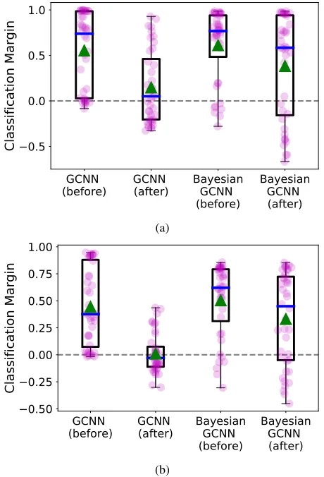
Figure 1 provides further insight concerning the impact of the attack on the two algorithms. The figure depicts the distribution of average classifier margins over the targeted nodes before and after the random attacks. Each circle in the figure shows the margin for one target node averaged over the 5 random perturbations of the graph. Note that some of the nodes have a negative margin prior to the random attack because we select the correctly classified nodes with lowest average margin based on 10 random trials and then perform another 5 random trials to generate the depicted graph. We see that for GCNN the attacks cause nearly half of the target nodes to be wrongly classified whereas there are consider-ably fewer prediction changes for the Bayesian GCNN.
GCNN
(before)
GCNN
(after)
Bayesian
GCNN
(before)
Bayesian
GCNN
(after)
0.5
0.0
0.5
1.0
Classification Margin
(a)
GCNN
(before)
GCNN
(after)
Bayesian
GCNN
(before)
Bayesian
GCNN
(after)
0.50
0.25
0.00
0.25
0.50
0.75
1.00
Classification Margin
(b)
Figure 1: Boxplots of the average classification margin for 40 nodes before and after random attacks for GCNN and Bayesian GCNN on (a) Cora dataset and (b) Citeseer dataset. The box indicates 25-75 percentiles; the triangle represents the mean value; and the median is shown by a horizontal line. Whiskers extend to the minimum and maxi-mum of data points.
6
Conclusions and Future Work
In this paper we have presented Bayesian graph convolu-tional neural networks, which provide an approach for in-corporating uncertain graph information through a paramet-ric random graph model. We provided an example of the framework for the case of an assortative mixed membership stochastic block model and explained how approximate in-ference can be performed using a combination of stochastic optimization (to obtain maximum a posteriori estimates of the random graph parameters) and approximate variational inference through Monte Carlo dropout (to sample weights from the Bayesian GCNN). We explored the performance of the Bayesian GCNN for the task of semi-supervised node classification and observed that the methodology improved upon state-of-the-art techniques, particularly for the case where the number of training labels is small. We also com-pared the robustness of Bayesian GCNNs and standard GC-NNs under an adversarial attack involving randomly chang-ing a subset of the edges of node. The Bayesian GCNN ap-pears to be considerably more resilient to attack.This paper represents a preliminary investigation into Bayesian graph convolutional neural networks and focuses on one type of graph model and one graph learning problem. In future work, we will expand the approach to other graph models and explore the suitability of the Bayesian frame-work for other learning tasks.
References
Airoldi, E. M.; Blei, D. M.; Fienberg, S. E.; and Xing, E. P. 2009. Mixed membership stochastic blockmodels. InProc. Adv. Neural Inf. Proc. Systems, 33–40.
Anirudh, R., and Thiagarajan, J. J. 2017. Bootstrapping graph convolutional neural networks for autism spectrum disorder classification. arXiv:1704.07487.
Atwood, J., and Towsley, D. 2016. Diffusion-convolutional neural networks. InProc. Adv. Neural Inf. Proc. Systems. Bresson, X., and Laurent, T. 2017. Residual gated graph convnets. arXiv:1711.07553.
Bruna, J.; Zaremba, W.; Szlam, A.; and LeCun, Y. 2013. Spectral networks and locally connected networks on graphs. InProc. Int. Conf. Learning Representations. Chen, J.; Ma, T.; and Xiao, C. 2018. FastGCN: fast learning with graph convolutional networks via importance sampling. InProc. Int. Conf. Learning Representations (ICLR). Defferrard, M.; Bresson, X.; and Vandergheynst, P. 2016. Convolutional neural networks on graphs with fast localized spectral filtering. InProc. Adv. Neural Inf. Proc. Systems. Denker, J. S., and Lecun, Y. 1991. Transforming neural-net output levels to probability distributions. InProc. Adv. Neural Inf. Proc. Systems.
Duvenaud, D.; Maclaurin, D.; et al. 2015. Convolutional networks on graphs for learning molecular fingerprints. In
Proc. Adv. Neural Inf. Proc. Systems.
Gal, Y., and Ghahramani, Z. 2016. Dropout as a Bayesian approximation: Representing model uncertainty in deep learning. InProc. Int. Conf. Machine Learning.
Goodfellow, I.; Shlens, J.; and Szegedy, C. 2015. Explain-ing and harnessExplain-ing adversarial examples. InProc. Int. Conf. Learning Representations.
Gopalan, P. K.; Gerrish, S.; et al. 2012. Scalable inference of overlapping communities. InProc. Adv. Neural Inf. Proc. Systems.
Hamilton, W.; Ying, R.; and Leskovec, J. 2017. Inductive representation learning on large graphs. InProc. Adv. Neural Inf. Proc. Systems.
Henaff, M.; Bruna, J.; and LeCun, Y. 2015. Deep convolutional networks on graph-structured data.
arXiv:1506.05163.
Hern´andez-Lobato, J. M., and Adams, R. 2015. Probabilis-tic backpropagation for scalable learning of Bayesian neural networks. InProc. Int. Conf. Machine Learning.
Kipf, T., and Welling, M. 2017. Semi-supervised classifica-tion with graph convoluclassifica-tional networks. InProc. Int. Conf. Learning Representations.
Korattikara, A.; Rathod, V.; Murphy, K.; and Welling, M. 2015. Bayesian dark knowledge. InProc. Adv. Neural Inf. Proc. Systems.
Levie, R.; Monti, F.; et al. 2017. Cayleynets: Graph convolu-tional neural networks with complex raconvolu-tional spectral filters.
arXiv:1705.07664.
Li, W.; Ahn, S.; and Welling, M. 2016. Scalable MCMC for mixed membership stochastic blockmodels. InProc. Artifi-cial Intelligence and Statistics, 723–731.
Li, C.; Chen, C.; Carlson, D.; and Carin, L. 2016a. Pre-conditioned stochastic gradient Langevin dynamics for deep neural networks. InProc. AAAI Conf. Artificial Intelligence. Li, Y.; Tarlow, D.; Brockschmidt, M.; and Zemel, R. 2016b. Gated graph sequence neural networks. InProc. Int. Conf. Learning Rep. (ICLR).
Liao, R.; Brockschmidt, M.; et al. 2018. Graph partition neural networks for semi-supervised classification. arXiv preprint arXiv:1803.06272.
Louizos, C., and Welling, M. 2017. Multiplicative nor-malizing flows for variational Bayesian neural networks.
arXiv:1703.01961.
MacKay, D. J. 1992. A practical Bayesian framework for backpropagation networks.Neural Comp.4(3):448–472.
MacKay, D. J. C. 1996. Maximum entropy and Bayesian methods. Springer Netherlands. chapter Hyperparameters: Optimize, or Integrate Out?, 43–59.
Monti, F.; Boscaini, D.; et al. 2017. Geometric deep learning on graphs and manifolds using mixture model CNNs. In
Proc. IEEE Conf. Comp. Vision and Pattern Recognition. Monti, F.; Shchur, O.; et al. 2018. Dual-primal graph con-volutional networks. arXiv:1806.00770.
Neal, R. M. 1993. Bayesian learning via stochastic dynam-ics. InProc. Adv. Neural Inf. Proc. Systems, 475–482.
Patterson, S., and Teh, Y. W. 2013. Stochastic gradient Rie-mannian Langevin dynamics on the probability simplex. In
Proc. Adv. Neural Inf. Proc. Systems.
Peixoto, T. P. 2017. Bayesian stochastic blockmodeling.
ArXiv e-print arXiv: 1705.10225.
Peng, L., and Carvalho, L. 2016. Bayesian degree-corrected stochastic blockmodels for community detection. Electron. J. Statist.10(2):2746–2779.
Scarselli, F.; Gori, M.; et al. 2009. The graph neural network model. IEEE Trans. Neural Networks20(1):61–80.
Sen, P.; Namata, G.; et al. 2008. Collective classification in network data. AI Magazine29(3):93.
Simonovsky, M., and Komodakis, N. 2017. Dynamic edge-conditioned filters in convolutional neural networks on graphs.arXiv:1704.02901.
Such, F.; Sah, S.; et al. 2017. Robust spatial filtering with graph convolutional neural networks. IEEE J. Sel. Topics Signal Proc.11(6):884–896.
Sukhbaatar, S.; Szlam, A.; and Fergus, R. 2016. Learning multiagent communication with backpropagation. InProc. Adv. Neural Inf. Proc. Systems, 2244–2252.
Sun, S.; Chen, C.; and Carin, L. 2017. Learning structured weight uncertainty in Bayesian neural networks. In Proc. Artificial Intelligence and Statistics.
Tishby, N.; Levin, E.; and Solla, S. 1989. Consistent in-ference of probabilities in layered networks: Predictions and generalization. InProc. Int. Joint Conf. Neural Networks. Veliˇckovi´c, P.; Cucurull, G.; Casanova, A.; Romero, A.; Li`o, P.; and Bengio, Y. 2018. Graph attention networks. InProc. Int. Conf. Learning Representations.
Yang, Z.; Cohen, W. W.; and Salakhutdinov, R. 2016. Re-visiting semi-supervised learning with graph embeddings.
arXiv preprint arXiv:1603.08861.