Three Parameter Laplace Type Bimodal Distribution

ISSN: 2231-5373

http://www.ijmttjournal.org

Page 352

Three Parameter Laplace Type Bimodal

Distribution

D V Ramana Murty1, G Arti2 and M. Vivekananda Murty3

1

Department of Statistics, VT College, Rajahmundry, East Godavari District, Andhra Pradesh, India.

2

Department of Management, GITAM (Deemed to be University), Visakhapatnam, India

3

Former Professor of Statistics, Andhra University, Visakhapatnam, India.

Abstract - This paper is on the Three parameter Laplace type Bimodal distribution. After discussing distributional properties, order statistics were developed and discussed. Inferential aspects were discussed and estimates of the parameters were obtained through Method of Moments and Maximum Likelihood Estimation techniques. Minimum unbiased estimator of the location parameter and best linear unbiased estimator of the location and scale parameter were also obtained.

I.INTRODUCTION

The Laplace distribution has received considerable attention as an appropriate model in reliability theory and life testing models.The statistical data in the fields like agriculture, meteorology and population studiesare appearing as if it is generated from a Laplace distribution, but have the kurtosis lies between 3 and 6. In this paper we introduce a three parameter Laplace type bimodal distribution which suits the distribution arising out of the situations mentioned above. The various distributional properties and inferential aspects of this distribution are discussed.

II. THREE PARAMETER LAPLACE TYPE BIMODAL DISTRIBUTION

A random variable is said to follow a three parameter Laplace type bimodal distribution, if its probability density function is of the following form.

𝑓 𝑥, 𝜇, 𝛽 =

𝑥−𝜇 𝛽

2𝑟

2𝛽 2𝑟 ! 𝑒

− 𝑥−𝜇_𝛽

, −∞< 𝑥 <∞, −∞< 𝜇 <∞, 𝛽 > 0 −→ 1

For different values of 𝑟 = 0,1,2, …∞ we have different continuous distributions with three parameters𝜇, 𝛽 and

𝑟(𝑟can be treated as an index parameter) which can be used to determine the specific distribution. This family includes Laplace distribution, when 𝑟 = 0[Johnson and Kotz (1972)]. Making the transformations,𝑦 =𝑥−𝜇_𝛽 in (1), we get

𝑓 𝑦 =_{2𝛽 2𝑟 !} 𝑦2𝑟𝑒−𝑦 , −∞< 𝑦 <∞ 2

The distribution given in (1) is symmetric about



and it is a generalized Laplace type distribution with three parameters.

III. PROPERTIES OF THREE PARAMETER LAPLACE TYPE BIMODAL DISTRIBUTION:

The distributions belonging to this family are having the following characteristics. The Mean of the distribution is

𝐸 𝑋 = 𝑥𝑓 𝑥, 𝜇, 𝛽 𝑑𝑥 = 𝑥

𝑥−𝜇 𝛽

2𝑟

2𝛽 2𝑟 ! 𝑒

− 𝑥−𝜇_𝛽

𝑑𝑥

∞

−∞ ∞

−∞

On simplification, one can get Mean = 𝜇

ISSN: 2231-5373

http://www.ijmttjournal.org

Page 353

𝑓(𝑥) 𝑑𝑥

𝑀 −∞

+ 𝑓(𝑥) 𝑑𝑥

∞

𝑀 = 1

𝑥

𝑥−𝜇 𝛽

2𝑟

2𝛽 2𝑟 ! 𝑒

− 𝑥−𝜇_𝛽

𝑑𝑥

𝑀 −∞

+ 𝑥

𝑥−𝜇 𝛽

2𝑟

2𝛽 2𝑟 ! 𝑒

− 𝑥−𝜇_𝛽

𝑑𝑥

∞

𝑀

= 1

Solving the equation one can have Median = 𝑀 = 𝜇

For the generalized three parameter Laplace type bimodal distribution, mean and median are equal.

For obtaining mode of the distribution, taking the derivatives of (1) with respect to

x

and equating to zero and solving for

x

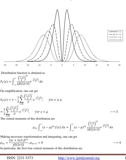
, we get the modes as𝜇 ± 2𝑟𝛽 ie. 𝜇 − 2𝛽and𝜇 + 2𝛽

Therefore, this distribution is bimodal.

Fig - 4.1

Distribution function is obtained as

𝐹𝑋(𝑥) =

𝑥−𝜇 𝛽

2𝑟

2𝛽 2𝑟 ! 𝑒

− 𝑥−𝜇_𝛽

𝑑𝑥

𝑥 −∞

On simplification, one can get

𝐹𝑋(𝑥) = 1 −

1 2

𝑥−𝜇 𝛽

𝑖

𝑖!

2𝑟

𝑖=0

𝑒− 𝑥−𝜇𝛽 _{, 𝑓𝑜𝑟 𝑥 ≥ 𝜇}

=1

2

𝑥−𝜇 𝛽

𝑖

𝑖!

2𝑟

𝑖=0

𝑒− 𝑥−𝜇𝛽 _{, 𝑓𝑜𝑟 𝑥 < 𝜇 −→ 3}

The central moments of this distribution are

𝜇2𝑛 𝑥 − 𝜇 2𝑛𝑓(𝑥) 𝑑𝑥

∞

−∞

= 𝑥 − 𝜇 2𝑛

𝑥−𝜇 𝛽

2𝑟

2𝛽 2𝑟 ! 𝑒

− 𝑥−𝜇_𝛽

𝑑𝑥

∞

−∞ Making necessary transformation and integrating, one can get

𝜇2𝑛 =

2𝑟 + 2𝑛 ! 𝛽2𝑛

𝛽 2𝑟 ! , 𝜇2𝑛+1= 0 −→ 4

In particular, the first four central moments of this distribution are

-25 -20 -15 -10 -5 0 5 10 15 20 25

ISSN: 2231-5373

http://www.ijmttjournal.org

Page 354

𝜇1= 0

𝜇2=

2𝑟 + 2 ! 𝛽2

2𝑟 !

𝜇3= 0

𝜇4=

2𝑟 + 4 ! 𝛽4

2𝑟 ! =

2𝑟 + 4 2𝑟 + 3 2𝑟 + 2 ! 𝛽4

2𝑟 !

Thus, the variance of this distribution is 𝜇2= 2𝑟+2 !𝛽

2

2𝑟 !

Since, the distribution is symmetric, its skewness is zero. The recurrence relation between the Central moments are

𝜇2𝑛 =

2𝑟 + 2𝑛 ! 𝛽2

𝛽 2𝑟 ! 𝜇2𝑛−2 −→ 5

The pth order absolute moments of the distribution are

𝐸 𝑋 − 𝜇 𝑝 _{= 𝑥 − 𝜇} 𝑝

𝑥−𝜇 𝛽

2𝑟

2𝛽 2𝑟 ! 𝑒

− 𝑥−𝜇_𝛽

𝑑𝑥

∞

−∞

On simplification, one can get,

𝐸 𝑋 − 𝜇 𝑝 ₌ 2𝑟 + 𝑝 ! 𝛽𝑝

2𝑟 ! −→ 6

The characteristic function of this distribution is

∅𝑋(𝑡) = 𝐸 𝑒𝑖𝑡𝑥 𝑒𝑖𝑡𝑥𝑓(𝑥) 𝑑𝑥 = 𝑒𝑖𝑡𝑥

𝑥−𝜇 𝛽

2𝑟

2𝛽 2𝑟 ! 𝑒

− 𝑥−𝜇_𝛽

𝑑𝑥

∞

−∞ ∞

−∞

Using the transformations 𝑦 = 𝑥 − 𝜇,and by simplification one can have

∅𝑋 𝑡 =

𝑒𝑖𝑡𝜇 _{2𝑟 !}

2

1

1 + 𝑖𝛽𝑡 2𝑟+1+

1

1 − 𝑖𝛽𝑡 2𝑟+1 −→ 7

Kurtosis of this distribution is

𝛽2=

𝜇4

𝜇22

𝑤𝑕𝑒𝑟𝑒 𝜇2=

2𝑟 + 2 ! 𝛽2

2𝑟 ! 𝑎𝑛𝑑 𝜇4=

2𝑟 + 4 ! 𝛽4

2𝑟 !

Therefore,𝛽2=(2𝑟+4) 2𝑟+3 _{2𝑟+2 !}

The distribution of the square of the variate:

Let 𝑌 = 𝑋2 and 𝛽 = 1, 𝜇 = 0, then the probability density function of

Y

is,

𝑓 𝑦 = 2𝑟 ! −2𝑟 _𝑦𝑖−1₂

𝑟

𝑖=0

𝑒− 𝑦_,

by transforming 𝑦 = 𝑧, 𝑓 𝑧 = _𝑟 2 2𝑟 ! −2𝑟

𝑖=0 𝑧2𝑖𝑒−𝑧,

Which is a mixture of𝛾- gamma variate with parameters 𝑧𝑖, 𝑖 = 0,1,2, … 𝑟. and weights

𝑤𝑖 = 2 2𝑖 ! 2𝑟 ! −2𝑟

IV. ORDER STATISTICS OF THREE PARAMETER LAPLACE TYPE BIMODAL DISTRIBUTION

The simple explicit form of the distribution function as given in (3) leads us to derive the Order statistics connected with this three parameter Laplace type bimodal distribution. For simplicity let us assume𝜇 = 0 𝑎𝑛𝑑 𝛽 = 1 then the probability density function (1) reduces to

𝑓 𝑥 = 𝑥 2𝑟𝑒− 𝑥

2 2𝑟 ! , −∞< 𝑥 <∞ −→ 8

Let 𝑋1:𝑛≤ 𝑋2:𝑛 ≤ ⋯ 𝑋𝑛:𝑛denote the Order statistics obtained from a random sample of size n from the standardized

Laplace type bimodal distribution having the probability density function of the form given (8). The probability density function of mth order statistics is given by

𝑓𝑚:𝑛 𝑥 = 𝐷𝑚:𝑛

𝑥 2𝑟_𝑒− 𝑥

2 2𝑟 !

𝑛 − 𝑚 𝑞

𝑛−𝑚

𝑞=0

(−1)𝑞 _{1 −}𝑒

−𝑥 _{2𝑟 !} 𝑥𝑖

𝑖!𝑒 − 𝑥 2𝑘 𝑖=0

2 2𝑟 !

𝑚+𝑞−1

ISSN: 2231-5373

http://www.ijmttjournal.org

Page 355

𝑓𝑚:𝑛 𝑥 = 𝐷𝑚:𝑛

𝑥 2𝑟_𝑒− 𝑥

2 2𝑟 !

𝑛 − 𝑚 𝑞

𝑛−𝑚

𝑞=0

(−1)𝑞 𝑒

−𝑥 _{2𝑟 !} 𝑥𝑖

𝑖!𝑒 − 𝑥 2𝑘 𝑖=0

2 2𝑟 !

𝑚+𝑞−1

𝑓𝑜𝑟 𝑥 < 0

Where 𝐷𝑚:𝑛 = 𝑚 𝑚_{𝑛 −→ 9}

The

a

th

moment of 𝑋𝑚:𝑛is given by

𝛼 𝑎 𝑚:𝑛

= 𝐷𝑚:𝑛 −1 𝑎

𝑛 − 𝑚 𝑞

𝑛−𝑚

𝑞=0

−1 𝑞 𝑚 + 𝑞 − 1

𝑗1 𝑚+𝑞−1

𝑗1>𝑗2>⋯𝑗𝑟

𝐷 0 𝑚 +𝑞−1−𝑗_{1 𝐷 𝑖} 𝑗_𝑖−𝑗_𝑖+1 𝑗𝑖

𝑗𝑖+1 𝑟−1

𝑖=1

𝐷 𝑟 𝑗_{𝑟 𝑃}

𝑗

𝑅!

(𝑚 + 𝑞)𝑅+1

𝑗

+𝐷′

𝑚:𝑛 𝑚 − 1_𝑙

𝑚−1

𝑙=0

−1 𝑙 𝑛 + 𝑙 − 𝑚

𝑗1 𝑛+𝑙−𝑚

𝑗₁>𝑗₂>⋯𝑗_𝑟

𝐷 0 𝑛+𝑙−𝑚−𝑗_{1 𝐷 𝑖} 𝑗_𝑖−𝑗_𝑖+1 𝑗𝑖

𝑗𝑖+1 𝑟−1

𝑖=1

𝐷 𝑟 𝑗_{𝑟 𝑃}

𝑗

𝑅!

(𝑛 + 𝑙 − 𝑚)𝑅+1

𝑗

Where 𝑅 = 𝑦=1𝑟 2𝑥=1𝑖 𝑗𝑥+ 2𝑟 + 𝑎, 𝐷′𝑚:𝑛=_{2 2𝑟 !}𝐷𝑚 :𝑛 , 𝐷 𝑟 =_{2 2𝑟 !} 2𝑟 !

And 𝑃𝑗 =

𝑎 𝑗𝑟1

𝑟−1 𝑟₁=1

𝑗𝑟_𝑖

𝑗𝑟_𝑖+1 2𝑟−1

𝑖=1 (𝑖)−𝑗𝑟𝑖 𝑗_𝑗2𝑟

1 2𝑟

𝑖=1 _𝑗𝑗𝑖

𝑖+1 (𝑖)

−𝑗_𝑖 2𝑟 𝑖=1 2𝑟−1

𝑖=1 −→ 10

From this (10) one can calculate the expected values of Order statistics.

Distribution of Median:

To obtain the distribution of Median, substitute 𝑚 =𝑛+1₂ if

n

is odd in (9). Thus, one can get

𝑓𝑛 +1

2 :𝑛 𝑥 = 𝐷𝑛 +12 :𝑛

𝑥 2𝑟_𝑒− 𝑥

2 2𝑟 !

𝑛 − 1 2 𝑞

𝑛 −1 2

𝑞=0

−1 𝑞 _{1 −}𝑒

− 𝑥 _{2𝑟 !} 𝑥𝑖

𝑖! 2𝑟 𝑖=0

2 2𝑟 !

𝑛 +2𝑞−1 2

𝑓𝑜𝑟 𝑥 ≥ 0

= 𝐷𝑛 +1

2 :𝑛

𝑥 2𝑟_𝑒− 𝑥

2 2𝑟 !

𝑛 − 1 2 𝑞

𝑛 −1 2

𝑞=0

−1 𝑞 𝑒

− 𝑥 _{2𝑟 !} 𝑥𝑖

𝑖! 2𝑟 𝑖=0

2 2𝑟 !

𝑛 +2𝑞−1 2

𝑓𝑜𝑟 𝑥 < 0

Where 𝐷𝑛 +1

2 :𝑛=

𝑛!

𝑛 −1₂ ! 2 11

when

n

is even then 𝑚 =2𝑛+1₄

𝑓2𝑛 +1

2 :𝑛 𝑥 = 𝐷

2𝑛 +1

2 :𝑛

𝑥2𝑟_𝑒− 𝑥

2 2𝑟 !

2𝑛 − 1 4 𝑞

2𝑛 −1 4

𝑞=0

−1 𝑞 _{1 −}𝑒

− 𝑥 _{2𝑟 !} 𝑥𝑖

𝑖! 2𝑟 𝑖=0

2 2𝑟 !

2𝑛 +4𝑞−3 4

𝑓𝑜𝑟 𝑥 ≥ 0

= 𝐷2𝑛 +1

2 :𝑛

𝑥2𝑟_𝑒− 𝑥

2 2𝑟 !

2𝑛 − 1 4 𝑞

2𝑛 −1 4

𝑞=0

−1 𝑞 𝑒

− 𝑥 _{2𝑟 !} 𝑥𝑖

𝑖! 2𝑟 𝑖=0

2 2𝑟 !

2𝑛 +4𝑞−3 4

𝑓𝑜𝑟 𝑥 < 0

12

Joint Moments of the Order Statistics

The joint probability distribution of the Order Statistics 𝑋𝑚:𝑛and 𝑋𝑠:𝑛, 𝑚 < 𝑠is given by

𝑓𝑚,𝑠:𝑛 𝑥 = 𝐷𝑚,𝑠:𝑛 𝑈 𝑥 𝑚−1 𝑈 𝑦 − 𝑈 𝑥 𝑠−𝑚−1 1 − 𝑈 𝑦 𝑛−𝑠𝑓 𝑥 𝑓(𝑦)

Where 𝑈 𝑥 =𝑥

2𝑟 _{2𝑟 !𝑒}− 𝑥 𝑥𝑖 𝑖! 2𝑟 𝑖=0

2 2𝑟 ! 13

Partition the range 0 < 𝑥 < 𝑦 <∞in to three mutually exclusive regions

𝑅1: 𝑥, 𝑦 : −∞< 𝑥 < 𝑦 < 0

𝑅2: 𝑥, 𝑦 : 0 < 𝑥 < 𝑦 <∞

𝑅3: 𝑥, 𝑦 : −∞< 𝑥 < 0, 0 < 𝑦 <∞

ISSN: 2231-5373

http://www.ijmttjournal.org

Page 356

𝐸[𝑋𝑚:𝑛, 𝑋𝑠:𝑛] = 𝑓 𝑥, 𝑦 𝑑𝑥𝑑𝑦

𝑅₁∪𝑅₂∪𝑅₃

= 𝐷𝑚,𝑠:𝑛 𝑠 − 𝑚 − 1_𝑖

𝑛 − 𝑠 𝑗

𝑛−𝑠

𝑗 =0 𝑠−𝑚−1

𝑖=0

−1 𝑠−𝑚−1+𝑖+𝑗_{Ψ 𝑠 − 2 − 𝑖, 𝑖 + 𝑗}

+ 𝑠 − 𝑚 − 1_𝑗 𝑚 − 1_𝑗

𝑠−𝑚−1

𝑗 =0 𝑚−1

𝑖=0

−1 𝑖+𝑗_{Ψ(𝑠 − 𝑚 − 1 + 𝑖 + 𝑗, 𝑛 − 𝑠 + 𝑗)}

− 𝑠 − 𝑚 − 1 − 𝑖_𝑗 𝑠 − 𝑚 − 1_𝑖

𝑛−𝑠

𝑗 =0 𝑠−𝑚−1

𝑖=0

−1 𝑖+𝑗 _{𝑥 𝑈 𝑥} 𝑚+𝑖−1_{𝑓 𝑥 𝑑𝑥 𝑦 𝑈 𝑦} ∞ 𝑛−𝑠−𝑗_{𝑓 𝑦 𝑑𝑦}

0 𝑥

0

where

Ψ 𝑎, 𝑏 = 𝑥𝑦 𝑈 𝑥 𝑦 𝑎

0

∞

0

𝑈 𝑦 𝑏_{𝑓 𝑥 𝑓 𝑦 𝑑𝑥𝑑𝑦}

= 2𝑟 !𝑦 −2

0

∞

0 𝑠 − 𝑚 − 1𝑣

𝑛 − 𝑠 𝑢

𝑛−𝑠

𝑢=0 𝑠−𝑚−1

𝑣=0

−1 𝑢+𝑣 _{𝑃 𝑗 𝑄(𝑡)} 𝑟

𝑁

𝑟

𝑁=0 𝑠−𝑚−1−𝑣−𝑢

𝑡 𝑚−𝑖+𝑣

𝑗

𝑒 𝑚−1+𝑣 𝑥+ 1−𝑚−1−𝑣+𝑢 𝑦_𝑥2𝑟+1+ 𝑟_𝑖=1 𝑗 𝑖_𝑙=0𝑗_𝑖𝑙𝑦2𝑟+1+ 𝑟_𝑖=1 2𝑖_𝑙=0𝑡_𝑖𝑙

𝑃 𝑗 = _𝑗𝑎

1

𝑗𝑖

𝑗𝑖+1 𝑟−1

𝑖=1

2𝑟 ! 𝑗𝑖−𝑗𝑖+1 𝑗𝑖− 𝑗𝑖+1

𝑗𝑖 2𝑟 !

𝑗𝑟 𝑗𝑖

𝑗𝑖+1 2𝑖−𝑗

𝑖=1 𝑟

𝑖=1

𝑙 −𝑗𝑖𝑙

2𝑖

𝑖=1

_𝑗𝑗𝑟

𝑟𝑙

𝑄 𝑡 = _𝑡𝑏

1

𝑡𝑖

𝑡𝑖+1 𝑟−1

𝑖=1

2𝑟 ! 𝑡_𝑖−𝑡_𝑖+1 𝑡𝑖− 𝑡𝑖+1

𝑡𝑖 2𝑟 !

𝑡𝑟 𝑡𝑖𝑙

𝑡𝑖𝑙+1 2𝑖−1

𝑙=1 𝑟

𝑖=1

𝑙 −𝑡_𝑖𝑙

2𝑖

𝑖=1

_𝑡𝑡𝑟

𝑟𝑙

14

V. ESTIMATION OF PARAMETERS:

Previously we have studied three parameter generalized Laplace type bimodal distribution and its distributional properties. Another aspect of any distributional study is to look in to the inferential aspects of the distribution, in particular the estimation of the parameters involved in the distribution under study. In this we will discuss the various methods of estimation by using Method of moments, maximum likelihood method of estimation, Best linear unbiased estimation in estimating the parameters of the three parameter Laplace type bimodal distribution and specially by using Numerical Analysis techniques namely Newton Raphson‟ s method & iterative method. The asymptotic behavior of these estimators is also studied. In this distribution the value of r is fixed, based on the Kurtosis of the distribution. After identifying r we estimate these moving parameters 𝜇and 𝛽.

A. Method of Moments:

According to this method, the moments of the population and the sample are equated correspondingly to deduce the estimators of the parameters. Let us consider a sample of size „n‟ drawn from a population having the probability density function of the form given by

𝑓(𝑥, 𝜇, 𝛽) =

𝑥−𝜇 𝛽

2𝑟

2𝛽 2𝑟 ! 𝑒

− 𝑥−𝜇_𝛽

This distribution is having two parameters𝜇 & 𝛽 and

r

is identified through the sample kurtosis. Hence, we consider the first two moments of the sample and the population, which leads to the following equations.

𝜇 = 𝑥,

2𝑟+2 ! 𝛽2

2𝑟 ! = 𝑠

2₌1

𝑛 𝑥𝑖− 𝑥

2 𝑛

𝑖=1 15

These equations give us the moment estimators as

ISSN: 2231-5373

http://www.ijmttjournal.org

Page 357

𝑎𝑛𝑑 𝛽 2₌ 2𝑟 ! 𝑠2

2𝑟 + 2 !

where 𝑠2 isthe sample variance. The variance of 𝜇 is

𝑉𝑎𝑟 𝑥 = 𝑉𝑎𝑟 1

𝑛 𝑥𝑖

𝑛

𝑖=1

= 1

𝑛2 𝑉𝑎𝑟 𝑥𝑖 =

1 𝑛2

2𝑟 ! 𝑠2 _𝛽2

2𝑟 + 2 !

𝑛

𝑖=1

= 𝛽

2

𝑛

2𝑟 + 2 !

2𝑟 ! → 16

𝑛

𝑖=1

and _𝑛1 𝑛𝑖=1𝐸(𝑥𝑖) = 𝜇

That is the sample mean is an unbiased estimator of𝜇17

The unbiased estimator of 𝛽2is 𝛽 2= _{2𝑟+2 !} 2𝑟 !𝑠2 18 where 𝑠2 is the sample variance.

The variance of the estimators are given by

𝑉𝑎𝑟 𝜇 = 𝛽_𝑛2 2𝑟+2 ! _{2𝑟 !} 19

and the unbiased estimator of 𝛽2,

𝑉𝑎𝑟 𝛽 = 𝛽2 4 2𝑟 !

2𝑟 + 2 !

2

2𝑟 + 4 ! _{2𝑟 !} 1

𝑛−

2

𝑛2−

1 𝑛3 −

2𝑟 + 4 ! 2𝑟 !

2

1

𝑛−

4

𝑛2−

3 𝑛3

20 As the variance tends to zero when n tends to



, the estimators 𝑥 and𝑠2are consistent for 𝜇 and 𝛽2 Similar to the simple Laplace distribution the median is the maximum likelihood estimators of the parameter 𝜇. Hence estimation of all the parameters can be done sequentially with𝜇being estimated by the median and then the other two parameters can be simultaneously estimated conditioned to 𝜇 = 𝜇

B. Maximum Likelihood Method of Estimation:

Let𝑥1, 𝑥2, … . 𝑥𝑛 be a sample of size n drawn from a population having the probability density function of

the form given in equation (1). From equation (1) one can write the likelihood function of the sample is

𝐿 =

𝑥−𝜇 𝛽

2𝑟

𝑒−

𝑥−𝜇 𝛽 𝑛

𝑖=1

2𝛽 2𝑟 ! 21

Taking logarithms on both sides of (4.6.1) we get

𝑙𝑜𝑔𝐿 = 𝑛 +2𝑟

𝛽

(𝑥𝑖− 𝜇)

𝑥_𝑖−𝜇 𝛽

2 −

𝑛

𝑖=0

1

𝛽 𝑥𝑖− 𝜇 = 0

𝑛

𝑖=1

−→ 22

For obtaining the maximum likelihood estimators of the parameters we have to maximize

L

or

log

L

with respect to the parameters𝜇 and𝛽. The values of 𝜇 and𝛽 can be obtained by solving the following equations.

2𝑟 !

2𝑟 + 2 !− 𝑟

1

𝑥_𝑖−𝜇 𝛽

2= 0

𝑛

𝑖=0

That is _{𝑥𝑖−𝜇}1 𝛽

2− 2𝛽 2𝑟 ! = 0

𝑛

𝑖=0 23

C. Best Linear Unbiased Estimators:

The best linear unbiased estimators of the location and scale parameters involved in the three parameter Laplace type bimodal distribution having the probability density function of the form given in (1) are obtained as follows. For that consider the family of distributions given in equation (1)

Let 𝑋𝑚:𝑛′ and𝑋𝑚:𝑛be the

m

th order statistics drawn from the populations having the probability density function of

the form given above and the corresponding standardized distribution respectively.

ie.𝑋𝑚:𝑛= 𝑋𝑚 :𝑛

′ _−𝜇

𝛽 , 1 ≤ 𝑚 ≤ 𝑛

ISSN: 2231-5373

http://www.ijmttjournal.org

Page 358

𝜇∗₌𝑙′Ω𝑋

𝑙′_Ω𝑙 𝑎𝑛𝑑 𝛽∗=

𝛼′_Ω𝑋

𝛼′_Ωα where 𝑙′= 1,1, … ,1 , 𝑋′= 𝑋1:𝑛, 𝑋2:𝑛, … 𝑋𝑛:𝑛 𝑎𝑛𝑑 𝛼′= 𝛼1:𝑛, 𝛼2:𝑛, … 𝛼𝑛:𝑛

where,𝛼1:𝑛is the first moment of the𝑖𝑡𝑕 order statistics and Ω is the variance matrix of vector

X

The variance of these estimators are 𝑣𝑎𝑟(𝜇∗) =_𝑙′𝜎_Ω𝑙, 𝑣𝑎𝑟 𝛽∗ =

𝜎

𝛼′_Ωαand 𝑐𝑜𝑣(𝜇∗, 𝛽∗) = 0

With the moments of the order statistics given in section 4 and 5, one can compute the𝜇∗and𝛽∗and their variances respectively.

REFERENCES:

[1] Cramer, H. (1946): Mathematical Methods of Statistics, Asia Publishing House. [2] David. H.A. (1981): Order Statistics, John Wiley & Sons, Ins. New York.

[3] Eisenberger, I. (1964): „Genesis of Bimodal distributions‟ techno metrics, p.357-363., vol.6.

[4] Feller, W. (1966). An Introduction to Probability Theory and Its Applications, Vol.I I, New York, John Wiley & sons, NC.

[5] Govindarajulu, Z. (1966): Best linear estimates under symmetric censoring of the parameters of a double exponential population, journal of the Statistical Association,61.

[6] Johnson, N.L. And kotz, S. (1970): Continuous Univariate Distributions, john Wiley Sons, New York. [7] Kameda, T. (1928): On the reduction of frequency curves, SckandinaviskAktuarietidskrift, 11.

[8] Laplace, P.S. (1774): Memoire sur la pobabilite des causes par les evenemens, Memoiries de mathematique et de Physique, 6. [9] Lloyd, E.H. (1952): Least square estimation of location and scale parameters using order statistics, Biometrica, 39.

[10] Rao, C.R. (1965): Linear Statistical Inference and its applications, Wiley Eastern. [11] Rao, K.S. et al. (1988): A bimodal distribution, Bulletin.Cal.math. Soc.,80, No.4.

[12] Sharma, P.V.S, Rao, K.S.S, And Rao, R.P (1990): “On a family of bimodal distributions” Sankhya 52,3,287-292.