An M/G/1 Feedback Queueing System with Second Optional Service and with Second Optional Vacation

Vol. 8, No. 2, 2015, 101-113

ISSN: 2320 –3242 (P), 2320 –3250 (online) Published on 6 October 2015

www.researchmathsci.org

101

An M/G/1 Feedback Queueing System with Second

Optional Service and with Second Optional Vacation

P.Manoharan1 and K.Sankara Sasi2 1

Department of Mathematics, Annamalai University, Annamalainagar-608 002 INDIA. E-mail: [email protected]

2

Department of Mathematics, Annamalai University, Annamalainagar-608 002 INDIA. E-mail: [email protected]

Received 1 June 2015; accepted 17 August 2015

Abstract.We study an M/G/1 queueing system with Bernoulli feedback and with second optional service and second optional vacation. Customers arrive singly and are served one by one according to FCFS rule. The service time follows general distribution. All arriving customers are provided first essential service, where as only some of them demand second service which is optional. After the completion of first or second service, if the customer is dissatisfied with service he can immediately join the tail of the queue as a feedback customer for receiving another regular service. Otherwise the customer may depart forever from the system. Soon after the system is empty the server takes a vacation and after returning from vacation the server may opt for second vacation based on a Bernoulli rule. Using supplementary variable technique, we derive the probability generating function for the number of customers in the system. Some performance measures are calculated. Some special cases and particular cases are discussed. A numerical study is also presented.

Keywords: M/G/1 queue, first essential service, second optional service, Bernoulli feedback, regular vacation, second optional vacation, steady state solution.

AMS Mathematics Subject Classification (2010): 60K25, 60K30 1. Introduction

102

correcting a major fault when the system is not in proper working condition. The organization of the paper is as follows. In section 2 the model is described. In section 3 the probability generating function for the number of customers in the system is derived. In section 4 some performance measures are calculated. In section 5 particular cases are discussed. In section 6 special cases are discussed and in section 7 a numerical study is presented. A conclusion is given in the last section.

2. The model

The following assumptions briefly describe the mathematical model of our study. The arrival follows Poisson distribution with mean arrival rate λ (> 0). There is a single server who provides the first essential service (FES) to all arriving customers. The service time for FES follows a general distribution, with distribution function B₁(x)and density functionb₁(x).

Immediately after the FES, the customer may opt with probability p for a second service which is optional (SOS), or he may leave the system with probability (1 − p), in which case another customer at the head of the queue (if any) is taken up for his FES. The service time for SOS is also assumed to be generally distributed. Let B₂(x) and

(x)

b₂ respectively be the distribution function and the density function of the SOS times. Further it is assumed that µ_i(x)dx is the conditional probability of completion of the ith service given that the elapsed service time is x so that

[

1 B(x)

]

(x) b (x)dx

µ

i i i

−

= and

thereforeb(x) µ (x)exp( ) ; i {1,2}

x

0 (t)dt i µ

i

i = −∫ ∈ .

We assume that the FES and SOS are mutually independent of each other. Let

1,2,3} { i 1), (k ) E(B (s),

B*_i k_i ≥ ∈ denote the LST and finite moments of two service times respectively. Thus the total service time required by the server to complete the service cycle which may be called as modified service period is given by

  

−

= +

p 1 y probabilit with

p y probabilit with

B

1 2 1

B B B

After the completion of first or second service, if the customer is dissatisfied with the service received to him, he can immediately join the tail of the queue as a feedback customer for receiving another regular service with probability r. Otherwise he may depart forever from the system with probability (1 – r) .

Whenever the system becomes empty, the server goes for a first regular vacation (FRV) of random lengthV1. Let V1(x)and v1(x) respectively be the distribution function

and density function of the first vacation times.

103

Further it is assumed that ν_i(x)dx is the conditional probability of the completion of the vacation given that the elapsed vacation time is

x

so that

(x) V 1

(x) v dx (x)

ν

i i i

−

= and

therefore ;

(t)dt

ν

e (x)

ν

(x) v

x

0 i i

i

∫

−

= i∈{1,2}.

It is also assumed that the vacation times V1 and V2are mutually independent of each

other having LSTs V_i*(s)and finite momentsE(V_ik),(k≥1), i∈{1,2}. Thus the total vacation time required to complete the vacation cycle, which may be called as modified vacation period is given by



 

− +

=

θ

1 y probabilit with

V

θ

y probabilit with

V V V

1 2 1

3. Queue size distribution at a random epoch

Here we first set up the steady state equations for the stationary queue size distribution by treating elapsed service time, FES time, SOS time, FRV time and SOV time as supplementary variables. Then we solve these equations and derive the PGF’s. Let N(t) be the queue size (including one being served, if any), B₁(0)(t)be the elapsed service time for FES, B(0)₂ (t) be the elapsed service time for the SOS, V₁(0)(t) be the elapsed vacation time for the FRV, V₂(0)(t) be the elapsed vacation time for the SOV at time t respectively. For further development of this model let us introduce the random variable Y (t) as follows.

      

=

t time at SOS giving busy is server the if 3

t time at FES giving busy is server the if 2

t time at SOV on is server the if 1

t time at FRV on is server the if 0

Y(t)

The supplementary variablesV₁(0)(t),V₂(0)(t);B₁(0)(t) , B₂(0)(t) are introduced in order to obtain a bivariate Markov process

{

N(t);∂(t);t≥0

}

where

 

  

 

= = = =

= ∂

3 Y(t) if (t) B

2 Y(t) if (t) B

1 Y(t) if (t) V

0 Y(t) if (t) V

(t)

(0) 2

(0) 1

(0) 2

(0) 1

We define the limiting probabilities as follows.

{

N(t) n; (t) V (t);x V (t) x dx

}

; n 0; x 0

Pr tlim (x)dx

Q_1,n = ∂ = ₁(0) < ₁(0) ≤ + ≥ >

∞ →

=

{

N(t) n; (t) V (t);x V (t) x dx

}

; n 0; x 0

Pr tlim (x)dx

Q_2,n = ∂ = ₂(0) < ₂(0) ≤ + ≥ >

∞ →

104

{

N(t) n; (t) B (t);x B (t) x dx

}

; n 0; x 0

Pr tlim (x)dx

P_1,n = ∂ = ₁(0) < ₁(0) ≤ + ≥ >

∞ →

=

{

N(t) n; (t) B (t);x B (t) x dx

}

; n 0; x 0

Pr tlim (x)dx

P_2,n = ∂ = (0)₂ < ₂(0) ≤ + ≥ >

∞ →

=

Further it is assumed that B (0) 0;Bi(0)( ) 1

(0)

i = ∞ = for i∈{1,2} and

1 ) ( V 0; (0)

V_i(0) = _i(0) ∞ = for i∈{1,2} and are continuous at x=0.

By assuming that the system is in steady state condition the differential difference equations governing the system are obtained as

(x)

λP (x) (x))P

µ

(λ

(x) P dx

d

1 1 1

1

1,n + + ,n = ,n− , x>0, n≥1

( )

1 0,

(x) (x))P

µ

(λ

(x) P dx

d

1,0 1

1,0 + + = x>0

( )

2

(x), ,

λP (x) , (x))P

µ

(λ

(x) P dx

d

1 2 2

2

2,n + + n = n− x>0, n≥1

( )

3 0,

(x) (x))P

µ

(λ

(x) P dx

d

2,0 2

2,0 + + = x>0

( )

4

(x), ,

λQ (x) , (x))Q

ν

(λ

(x) , Q dx

d

1 1 1

1

1n + + n = n− x>0, n≥1

( )

5 0,

(x) (x))Q

ν

(λ

(x) Q dx

d

1,0 1

1,0 + + = x >0

( )

6

(x), ,

λQ (x) , (x))Q

ν

(λ

(x) , Q dx

d

1 2 2

2

2n + + n = n− x>0, n≥1

( )

7 0,

(x) (x))Q

ν

(λ

(x) Q dx

d

2,0 2

2,0 + + = x>0,

( )

8 ∫

− +

∫

− −

= ∞ ∞

0

2 2,0 0

1 1,0

1,0 (1 p)(1 r) P (x)µ (x)dx (1 r) P (x)µ (x)dx λQ

(1 θ) Q (x)ν (x)dx Q (x)ν₂(x)dx

0 2,0 0

1

1,0 +∫

∫

−

+ ∞ ∞

( )

9

where

( )

∫

=∞

0 1,0 1,0 Q x dx

Q

The boundary conditions are

1,0 1,0(0) λQ

Q = (10)

0, (0) ,

Q_1n = n≥1 (11)

∫

= ∞

0

1 1

2, (0) θ Q, (x)ν (x)dx,

Q _{n n} n≥0

( )

12

∫ + − − ∫

+

∫

−

= ∞ ∞ ∞

0 0

1 1,1 2

2,0 0

1 1,0

1,0(0) r(1 p) P (x)µ (x)dx P (x)µ (x)dx (1 r)(1 p) P (x)µ (x)dx

105

( )

13 (x)dx

(x)ν

Q (x)dx (x)ν

Q

θ) (1 (x)dx (x)µ

P r) (1

0

2 2,1 1

0 1,1 0

2

2,1 + − ∫ +∫

∫

−

+ ∞ ∞ ∞

∫ + − − ∫ ₊

+

∫

−

= ∞ ∞ ∞

0 0

1 1 1 2

2 0

1 1

1, (0) r(1 p) P, (x)µ (x)dx P, (x)µ (x)dx (1 r)(1 p) P, (x)µ (x)dx

P _{n n n n}

(14) 1 n , (x)dx (x)ν

, Q (x)dx (x)ν

, Q

θ) (1 (x)dx (x)µ

, P r) (1

0

2 1 2 1

0 1 1 0

1

2n 2 + − ∫ n+ +∫ n+ ≥

∫ ₊

−

+ ∞ ∞ ∞

(x)dx, (x)µ

, P p (0) ,

P ₁

0 1 2n = ∫ n

∞

n≥0 (15)

and the normalizing condition is 1 i Q (x)dx (x)dx

P

0 2

10 1

2

10 n i,n

n i i,n =

∑ ∑

=∫ +

∑

= ∑=∫

∞ ∞ ∞

= ∞

(16)

Now let us define the following PGF’s

(x); P z z) (x,

P _i,n

n n i

0 ∑

=

= ∞ x≥0, z ≤1, i∈

{ }

1,2 (17)

(0); P z z) (0,

P _i,n

n n i

0 ∑

=

= ∞ z ≤1, i∈

{

1,2} (18)

(x); Q z z) (x,

Q _i,n

n n i

0 ∑

=

= ∞ x≥0, z ≤1, i∈

{

1,2

}

(19)

); ( Q z z) , (

Q _i,n 0

n n 0

i

0 ∑

=

= ∞ z ≤1, i∈

{

1,2

}

(20)

∫

=∞

0

z)dx, (x, P (z)

P_{i i} i∈

{

1,2} (21)

z)dx, (x, Q (z) Q

0 i

i = ∫

∞

i∈

{

1,2

}

(22)

Multiplying (1) by zn and summing over n=1 to

∞

and adding with (2), we get 0

z) (x, P ) (x)

µ λz

λ

( z) (x, P dx

d

1 1

1 + − + =

z)x λ(1 e ] (x) B 1 [ z) (0, P z) (x,

P₁ = ₁ − ₁ − − (23)

Multiplying (3) by zn and summing over n=1 to

∞

and adding with (4), we get 0

z) (x, P ) (x)

µ λz

λ

( z) (x, P dx

d

2 2

2 + − + =

z)x λ(1 (x)]e B z)[1 (0, P z) (x,

P₂ = ₂ − ₂ − − (24)

Multiplying (5) by zn and summing over n=1 to

∞

and adding with (6), we get 0

z) (x, Q ) (x)

ν λz

λ

( z) (x, Q dx

d

1 1

1 + − + =

z)x λ(1 e (x)] V z)[1 (0, Q z) (x,

Q₁ = ₁ − ₁ − − (25)

106 0 z) (x, Q ) (x) ν λz λ ( z) (x, Q dx d 2 2

2 + − + =

z)x λ(1 (x)]e V z)[1 (0, Q z) (x,

Q₂ = ₂ − ₂ − − (26)

Multiplying (14) by zn+1 and summing over n=1 to

∞

and adding with z times (13), we get

( )

1 z] P(x,z)µ (x)dx [1 r

( )

1 z] P (x,z)µ (x)dx r p)[1 (1 z) (0, zP ₂ 0 2 1 0 1

1 = − − − ∫ + − − ∫

∞ ∞ 2 1,0 0 2 1 0

1(x,z)ν (x)dx Q (x,z)ν (x)dx λQ

Q

θ)

(1− ∫ +∫ −

+ ∞ ∞ (27)

From equation (15), we get

λz) (λ z)B (0, pP z) (0,

P₂ = ₁ *₁ − (28) From equation (23), we get

λz) (λ z)B (0, P (x)dx z)µ (x,

P _{1 1} *₁

0

1 = −

∫

∞

(29)

From equation (24), we get

λz) (λ λz)B (λ z)B (0, pP (x)dx z)µ (x,

P *2

* 1 1 2

0

2 = − −

∫

∞

(30)

From equation (25), we get λz) (λ z)V (0, Q (x)dx z)ν (x,

Q _{1 1 1}*

0

1 = −

∫

∞

(31)

From equation (26), we get

λz) (λ λz)V (λ z)V (0, Q θ (x)dx z)ν (x,

Q 2*

* 1 1 2

0

2 = − −

∫

∞

(32)

From equation (11) and (12), we get

1,0 1(0,z) λQ

Q =

(33)

λz) (λ z)V (0, Q θ z) (0,

Q₂ = _{1 1}* − (34) Using (28) to (34) in (27), we get

( )

{

}

1,0 * 1 * 2 * 1 * 2 1 Q ] z) r(1 1 [ λz) (λ B λz)] (λ pB p) [(1 z 1 λz) (λ V λz)] (λ V θ θ 1 [ λ z) (0, P _      − − − − + − − − − − + −

= (35)

Using (35) in (28), we get

{

}

1,0 * 1 * 2 * 1 * 1 * 2 2 Q ] z) r(1 1 [ λz) (λ B λz)] (λ pB p) [(1 z λz) (λ B 1 λz) (λ V ] λz) (λ V θ θ) 1 ( [ pλ z) (0, P _      − − − − + − − − − − − + −

= (36)

Integrating (23) to (26) between 0 and ∞, we get z) (0, P λz) (λ λz) (λ B 1 (z) P ₁ * 1 1       − − − = (37) z) (0, λz)P (λ B λz) (λ λz) (λ B 1 p (z)

P ₁* ₁

107 z) (0, Q λz) (λ λz) (λ V 1 (z) Q ₁ * 1 1       − − − = (39) z) (0, Q λz) (λ λz)] (λ V λz)[1 -(λ θV (z) Q ₁ * 1 * 2 2       − − − = (40)

Using (35) in (37) and (38), we get

1.0 * 1 * 2 * 1 * 1 * 2 1 Q } ] z) 1 ( r 1 [ λz) (λ B λz)] (λ pB p) [(1 z){z (1 ) λz) (λ B 1 ( } 1 λz) (λ V ] λz) (λ θV θ) (1 [ { (z) P

_











− − − − + − − − − − − − − + − = (41)

{

}

( )

{

_*

}

_1.0

( )

42

1 * 2 * 1 * 2 * 1 * 2 2 Q ] z 1 r 1 [ λz) (λ B λz)] (λ pB p) [(1 z z) (1 λz) (λ B ) λz) (λ B 1 ( 1 -λz) (λ V ] λz) (λ θV θ) (1 [ p (z) P

_











− − − − + − − − − − − − − + − =

Using (33) in (39) and (40), we get

1,0 * 1 1 Q ) z 1 ( λz) (λ V 1 (z) Q _      − − −

= (43)

1,0 * 2 * 1 2 Q ) z 1 ( λz)] (λ V λz)[1 (λ θV (z) Q

_











− − − −

= (44)

Using the fact thatP₁(1)+P₂(1)+Q₁(1)+Q₂(1)=1 , we arrived

[

E(V) θE(V )

]

r) λ(1 ρ 1 Q 2 1 1,0 + − −

= (45)

where )] pE(B ) λ[E(B r

ρ= + ₁ + ₂

( )

46

and B*₁ (0) E(B₁), B*₂(0) E(B₂),

' '

− = −

= are the mean of service times of FES and SOS time respectively, V (0) E(V₁)

' *

1 =− and V (0) E(V2) '

*

2 =− are the mean of vacation times of FRV

and SOV respectively. Therefore

D(Z) N(Z)

P(z)=

( )

47

where

{

}{

}

1,0

* 1 * 2 * 1 *

2(λ λz)]V (λ λz) 1 1 [(1 p) pB (λ λz)]B (λ λz)rQ

θV

θ) [(1

N(z)= − + − − − − − + − −

{

z [(1 p) pB (λ λz)]B (λ λz)

}

[1 r(1 z)]

D(z) 1*

*

2 − − − −

+ − − =

4. Performance measures

Let Lqand L denote the steady state average queue size and system size respectively.

108 Using the L’Hospital rule twice we obtain

2

(1)) ' 2(D

(1) '' (1)D ' N (1) '' (1)N ' D

L_q = − (48)

where

1,0 2

1) θE(V))(1 r)Q

λ(E(V (1)

N' = + −

{

1 2 1 2 1 2

}

1,0

2 2 2

1 2

Q )) pE(B ) ))(E(B

θE(V ) 2r(E(V r)

)](1 )E(V E(V

θ

2 )

θE(V ) [E(V

λ

(1)

N'' =− + + − − + +

(

E(B) pE(B )

)

λ

r 1 (1)

D' = − − ₁ + ₂

{

E(B ) pE(B )

}

r λ

{

E(B ) pE(B ) 2pE(B )E(B )

}

2λ

(1)

D'' =− ₁ + ₂ − 2 ₁2 + 2₂ + _{1 2}

where E(B₁2),E(B2₂),E(V₁2),E(V₂2) are second moment of FES, SOS, FRV and SOV time

respectively. Next, we can obtainL=L_q +ρ, where L_q and ρ have been found in (48) and (46) respectively. Then using Little’s formulae, we obtain W_q,the average waiting time in the queue and W, the average waiting time in the system, as

λ

L W_q = q and

λ

L

W= respectively.

5. Particular cases

Case 1: Setting r =0 ( no feedback ) in (47) , we get

1,0 2 1

* 1 *

2

* 1 *

2

Q )]

θE(V )

λ[E(V }

λz) (λ

B ]

λz) (λ

pB ) p 1 ( [ z {

ρ) (1 } 1

λz) (λ

V ]

λz) (λ θV

θ) (1 {[ P(z)

+ −

− +

− −

− − − −

+ −

=

which coincides with the PGF of Manoharan [10] irrespective of the notations used . Case 2: Setting p=0 (no SOS) and r=0 (no feedback) in (47) we

get _1,0

2 1

* 1

* 1 *

2

Q ] ) E(V

θ

) E(V [

λ λz)} (λ

B z {

ρ) (1 } 1

λz) (λ

V ]

λz) (λ θV

θ) (1 [ { P(z)

+ −

−

− − − −

+ −

=

which coincides with the PGF of Choudhury [4] irrespective of the notations used. 6. Special cases

For validating our model it is important to analyze through specific distribution. By choosing some known distributions for service times and vacation times the validity of the system is examined in this section.

Model-1: Let the distribution of service and vacation times be assumed as Exponential. Then equations (45), (46), (47), (48) and (49) become

2 1

1 2 2 1

µ µ

) pµ λ(µ µ

rµ

ρ= + +

)

θν λ(ν µ

r)µ

(1

ν ν

) ) pµ λ(µ

r) (1

µ µ

( Q

1 2 2 1

2 1 1 2 2

1 1,0

+ −

109

(

)(

)

(

)

(

)

1,0

2 1 1 2 2 1 2 1 1 1 2 1 1 1 2 Q ) ν λz λ )( ν λz λ )}( z) r(1 1 ( µ ] pµ µ λz λ p) (1 [ ) µ λz )(λ µ λz z(λ { } r µ λz λ p ]] r µ µ λz λ [ µ λz λ [

λz)ν θ(λ )] ν λz λ ( ν )[ ν λz λ {( P(z) + − + − − − + + − − − + − + − − + − + − + − − − + − − + − = 1,0 2 ) 1 2 2 1 ( 2 2 2 1 2 1 2 1 2 2 1 2 2 1 2 1 1 2 2 1 1 2 1 2 2 1 2 1 2 1 2 2 1 2 2 1 2 Q ) pµ λ(µ r) (1 µ µ ν ν )} µ pµ pµ λ(µ ) pµ (µ µ {rµ ν r)ν )(1 θν (ν } ν )ν pµ )(µ θν r(ν r) (1 µ ]µ ν θν θν {[ν ] ) pµ λ(µ r) (1 µ µ [ λ L_q + − − + + + + − + + + + − − + + + − − =           1,0 2 ) 1 2 2 1 ( 2 2 2 1 2 1 2 1 2 2 1 2 2 1 2 1 1 2 2 1 1 2 1 2 2 1 2 1 2 1 2 2 1 2 2 1 Q ) pµ λ(µ r) (1 µ µ ν ν )} µ pµ pµ λ(µ ) pµ (µ µ {rµ ν r)ν )(1 θν (ν } ν )ν pµ )(µ θν r(ν r) (1 µ ]µ ν θν θν {[ν ] ) pµ λ(µ r) (1 µ µ [ λ W_q + − − + + + + − + + + + − − + + + − − =          

Model-II: Let the service and vacation times be taken as Erlang distributions. Then equations (45), (46), (47), (48) and (49) become

2 1 1 2 2 1 µ µ ) pµ λ(µ µ µ r ρ= + +

(

)

1,0 2 1 2 1 1 1 2 2 1 1 1 2 1 2 1 k 1 2 Q k) ν λz (λ k) ν λz z))}(λ r(1 (1 k) (µ k) p(µ z))] r(1 (1 k) p)(µ (1 k) µ λz [z(λ k) µ λz {(λ r} k) (µ k) p(µ r] k) p)(µ (1 k) µ λz [(λ k µ λz λ { } k) (ν k) θ(ν ] k) ν λz (λ k) θ)(ν [(1 k) ν λz {(λ P(z) k k k k k k k k k k k k k k k k                 + − + − − − − − − − − + − + − − − − + − + − × + + − − − + − =

(

)

(

)

2 1,0

1 2 2 1 2 2 2 1 2 1 2 1 2 1 2 1 2 2 1 2 2 1 1 2 2 1 1 2 1 2 2 1 2 1 2 1 2 2 2 1 1 2 2 1 2 Q pµ µ λ r) (1 µ µ ν 2kν ν ]}ν µ 2pµ 1)µ p(k 1)µ p(k 1)µ λ[(k )r pµ (µ µ r){2kµ )(1 θν (ν µ )}µ pµ )(µ θν (ν ν 2rkν k] ν ν θ 2 1)ν θ(k 1)ν r)[(k (1 µ )]{µ pµ λ(µ µ r)µ [(1 λ q L + − − + + + + + + − + − + + + + − + + + + − + − − =                    

(

)

(

)

2 1,0

1 2 2 1 2 2 2 1 2 1 2 1 2 1 2 1 2 2 1 2 2 1 1 2 2 1 1 2 1 2 2 1 2 1 2 1 2 2 2 1 1 2 2 1 Q pµ µ λ r) (1 µ µ ν 2kν ν ]}ν µ 2pµ 1)µ p(k 1)µ p(k 1)µ λ[(k )r pµ (µ µ r){2kµ )(1 θν (ν µ )}µ pµ )(µ θν (ν ν 2rkν k] ν ν θ 2 1)ν θ(k 1)ν r)[(k (1 µ )]{µ pµ λ(µ µ r)µ [(1 λ q W + − − + + + + + + − + − + + + + − + + + + − + − − =                    

7. Numerical results

Assigning particular values to the parameters of the system as p=0.02, µ₁ =2.5, 1.5,

110

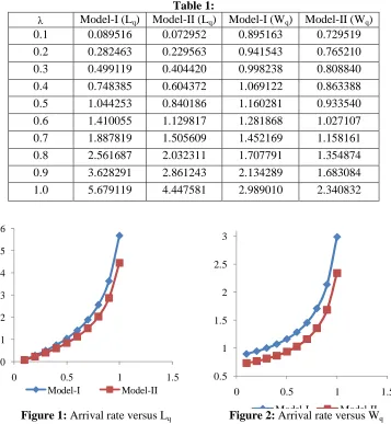
of 0.1 we calculated the values of Lq and Wq which are tabulated in Table-1 and the corresponding graphs are drawn for Model-I and Model-II in Figure 1 and Figure 2 respectively. We observe that when λ increases, there is a steady increase in Lq as well as in Wq for both Model-I and Model-II as can be expected.

Table 1:

λ Model-I (Lq) Model-II (Lq) Model-I (Wq) Model-II (Wq)

0.1 0.089516 0.072952 0.895163 0.729519

0.2 0.282463 0.229563 0.941543 0.765210

0.3 0.499119 0.404420 0.998238 0.808840

0.4 0.748385 0.604372 1.069122 0.863388

0.5 1.044253 0.840186 1.160281 0.933540

0.6 1.410055 1.129817 1.281868 1.027107

0.7 1.887819 1.505609 1.452169 1.158161

0.8 2.561687 2.032311 1.707791 1.354874

0.9 3.628291 2.861243 2.134289 1.683084

1.0 5.679119 4.447581 2.989010 2.340832

0 1 2 3 4 5 6

0 0.5 1 1.5

Model-I Model-II

0.5 1 1.5 2 2.5 3

0 0.5 1 1.5

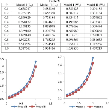
111 Table 2:

P Model-I (Lq) Model-II (Lq) Model-I (Wq) Model-II (Wq)

0.1 0.678247 0.582366 0.339123 0.291183

0.2 0.765035 0.662368 0.382517 0.331184

0.3 0.869829 0.758184 0.434915 0.379092

0.4 0.998172 0.874681 0.499086 0.437341

0.5 1.158135 1.018948 0.579068 0.509474

0.6 1.369160 1.201736 0.680980 0.600868

0.7 1.629140 1.440166 0.814570 0.720083

0.8 1.992731 1.763265 0.996366 0.881633

0.9 2.513624 2.224513 1.256812 1.112256

1.0 3.317661 2.934426 1.658830 1.467213

0.5 1 1.5 2 2.5 3 3.5

0 0.5 1 1.5

Model I Model II

0.2 0.5 0.8 1.1 1.4 1.7

0 0.5 1 1.5

Model I Model II

Figure 3: (probability of SOS) versus Figure4: (probability of SOS) versus

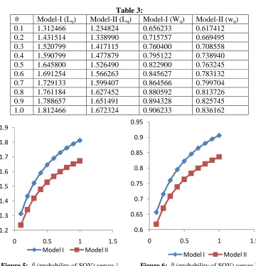
Taking the values of the parameters of as λ=2, p = 0.2, µ₁ =9, µ₂ =8, ν₁ =4,

2

ν =2, r =0.5 and varying the value of θ _{from 0.1 to 1 in steps of 0.1 we calculated the}

values of Lq and Wq which are tabulated in Table-3 and the corresponding graphs are drawn for Model-I and Model-II in Figure 5 and Figure 6 respectively. We observe that when θ increases, there is a steady increase in Lq and Wq for both Model-I and Model-II as can be expected.

112 Table 3:

θ Model-I (Lq) Model-II (Lq) Model-I (Wq) Model-II (wq)

0.1 1.312466 1.234824 0.656233 0.617412

0.2 1.431514 1.338990 0.715757 0.669495

0.3 1.520799 1.417115 0.760400 0.708558

0.4 1.590799 1.477879 0.795122 0.738940

0.5 1.645800 1.526490 0.822900 0.763245

0.6 1.691254 1.566263 0.845627 0.783132

0.7 1.729133 1.599407 0.864566 0.799704

0.8 1.761184 1.627452 0.880592 0.813726

0.9 1.788657 1.651491 0.894328 0.825745

1.0 1.812466 1.672324 0.906233 0.836162

1.2 1.3 1.4 1.5 1.6 1.7 1.8 1.9

0 0.5 1 1.5

Model I Model II

0.6 0.65 0.7 0.75 0.8 0.85 0.9 0.95

0 0.5 1 1.5

Model I Model II

Figure 5: (probability of SOV) versus Figure 6: (probability of SOV) versus

8. Conclusion

The analysis carried out in “An M/G/1 feedback Queueing system with second optional service and with second optional vacation” is to obtain the probability generating function for the number of customers in the system and also to obtain waiting time of a customer in the system. Numerical work is carried out to study the effect of some parameters on the operating characteristics of the system.

Acknowledgement. The second author thanks the UGC for proceeding and supporting the research work.

REFERENCES

113

2. G.Choudhury, Some aspects of an M/G/1 queueing system with second optional service, TOP, 11(1) (2003) 141-150.

3. G.Choudhury and M.Paul, A two phase queueing system with Bernoulli feedback, Information and Management Sciences, 16(1) (2005) 773-784.

4. G. Choudhury, An M/G/1 queue with an optional second vacation, Information and Management Sciences, 17(3) (2006) 19-30.

5. R.L.Disney, C.D.Mcnickle and B.Simon, The M/G/1 queue with instantaneous Bernoulli feedback, Naval Research Logist Quart, 27 (1980) 635-644.

6. R.Kalyanaraman and S.Pazhani Bala Murugan, A single server queue with additional optional service in batches and server vacation, Applied Mathematical Sciences, 2 (2008) 2765-2776.

7. B.Krishna Kumar, A.Vijayakumar and D.Arivudainambi, An M/G/1 retrial queueing system with two phase service and preemptive resume, Ann. Oper. Res, 113 (2002) 61 -79.

8. K.C.Madan, An M/G/1 queueing system with compulsory server vacations, Trabajos de Investigacion, 7 (1992) 105-115.

9. K.C.Madan, An M/G/1 queue with second optional service, Queueing Systems, 34 (2000) 37-46.

10. P.Manoharan and K.Sankara Sasi, An M/G/1 queue with Second optional service and with second optional vacation, Annamalai University Sci. Journal, 1 (2015) 15-22. 11. J.Medhi, A single server poisson input queue with a second optional service,

Queueing Systems, 42 (2002) 239-242.

12. V.Thangaraj, and S.Vanitha, A two phase M/G/1 feedback queue with multiple server vacation, Stochastic Analysis and Applications, 27 (2009) 1231-1245.