Modified Numerical Method for Solving Fredholm Integral Equations

(1)

Vol. 16, 2019, 67-76

ISSN: 2349-0632 (P), 2349-0640 (online) Published 22 April 2019

www.researchmathsci.org

DOI: http://dx.doi.org/10.22457/jmi.136av16a6

67

Journal of

Modified Numerical Method for Solving Fredholm

Integral Equations

Mazin H. Suhhiem and Mohammed H. Lafta Department of Statistics, University of Sumer, Alrifaee, Iraq

Email: [email protected]

Received 19 March 2019; accepted 21 April 2019

Abstract. In this work, we have presented a novel method to find the numerical solution of the linear Ferdholm integral equation of second kind. This method is based on the Taylor series multiplied by an exponential function to approximate the kernel as a summation of multiplication functions. The presented method has high accurate when compare its results with the other numerical methods results.

Keywords: Fredholm integral equation, Taylor series, degenerate kernel, analytical solution, numerical solution

AMS Mathematics Subject Classification (2010):45B05

1. Introduction

Integral equations, that is, equations involving an unknown function which appear under an integral sign. Such equations occur widely in divers areas of applied mathematics, they offer a powerful technique for using the integral equation rather than differential equations is that all of the conditions specifying the initial value problems or boundary value problems for a differential equation can often be condensed into a single integral equation. So that any boundary value problems can be transformed into Fredholm integral equation involving an unknown function of only once variable.

This reduction of what may represent a complicated mathematical model of physical situation into a single equation is itself a significant step, but there are other advantages to be gained by replacing differentiation with integration, some of these advantages arise because integration is a smooth process, a feature which has significant implication when approximation solution are sough.

(2)

68

In this work, we have introduced a modified numerical method for solving linear

Ferdholm integral equation of second kind: = +

∫

b

a

t y t x k x

f x

y( ) ( )

λ

( , ) ( )dt. This

method is based on Taylor series multiplied by the exponential function of (xt) to approximate the kernel k( tx, ) as a summation of multiplication functions fn(x) by

) (t

g_n i.e.

∑

=

= N

n

n n xg t f t x k

1

) ( ) ( )

,

( , then use the degenerate kernel idea to solve the

Fredholm integral equation .In this work we have solved the Fredholm integral equation with a=0and b=1,

λ

is a real number, f(x) and k( tx, ) are real continues functions.

2. Degenerate kernel [1]

A kernel k( tx, ) is called separable (degenerate) if it can be expressed as the sum of a

finite number of terms, each of which is the product of a function of x only and a

function of t only,

i.e.

∑

=

= n

i

i i x h t g

t x k

1

) ( ) ( )

,

( .

3. Solution of Ferdholm integral equation of second kind with degenerate kernel [1,2]

Consider the non-homogenous Fredholm integral equation of second kind :

dt t y t x k x

f x y

b

a

∫

+

= ( ) ( , ) ( )

)

(

λ

(1)

Since the kernel k( tx, ) is degenerate or separate we take :

∑

=

= n

i

i i x g t f

t x k

1

) ( ) ( )

,

( (2)

where the functions f_i(x) assumed to be linearly independent, From (1) and (2), we get

dt t y t g x f x

f x y

b

a n

i

i i

∫ ∑

=

+ =

1

) ( )] ( ) ( [ ) ( )

(

λ

(3)

or

∑

∫

=

+

= n

i

b

a i

i x g t y t dt f

x f x y

1

) ) ( ) ( ) ( )

( )

(

λ

(4)

From (3) and (4), we get

∑

=

+

= n

i i if x C x

f x y

1

)) ( )

( )

(3)

Mazin H. Suhhiem and Mohammed H. Lafta

69

where the constants Ci(i=1,2,3,...,n)are to be determined in order to find the solution of (1) in the form given by (5) .

We now proceed to evaluate Ci's as follows: From (5) we have

∑

= + = n i i if t C t f t y 1 )) ( ) ( )

(

λ

(6)

Substituting the values of y(x)and y(t)given in (5) and (6) respectively in (3), we have

∑

∫

∑

= = = + + = + n i n i b a n i i i i i i

if x f x f x g t f t C f t dt

C x

f

1 1 1

)} ( ) ( ){ ( ) ( ) ( ) ( )

(

λ

(7a)

or

∑

∫

∑

∫

= = = + = n i n i b a n j b a j i j j i i

if x f x g t f t dt C g t f t dt C

1 1 1

} ) ( ) ( ) ( ) ( ){ ( )

(

λ

(7b)

Now, let

=

∫

b

a i

i g (t) f (t)dt

β (8a)

And

∫

=b a j i

ij g (t)f (t)dt

α

(8b)

where

β

iand

α

ij are known constant, then (7) may simplify as :

∑

= = = + = n i n i n j j ij i i i

if x f x C

C

1 1 1

} ){

( )

(

β

λ

α

or

∑

= = = − − n i n j j ij i i

ix C C

f

1 1

0 } ){

(

β

λ

α

(9a)

but the functions fi(x)are linearly independent, therefore, we can write:

∑

= = − − n j j ij i i C C 1 0

α

λ

β

i=1,2,3,...,n (9b)

or

∑

= = − n j i j ij i C C 1

β

α

λ

i=1,2,3,...,n (9c)

Then we obtain the following system of linear equations to determine C1,C2,...,Cn

(4)

70 The determinate D(

λ

)of system

nn n

n

n n

D

λα

λ

− −

−

− −

−

− −

−

=

1 1

1

) (

2 1

2 22

21

1 12

11

… ⋮ ⋮

⋮ ⋮

… …

(10)

which is a polynomial in

λ

of degree at most (n), D(

λ

)is not identically zero, since when

λ

=0,D(

λ

)=1.to discuss the solution of (1), the following situation arise:

Situation I:

When at least on right member of the system (

β

1),(

β

2),....,(

β

n)is non zero, the following two cases arise under this situation :

(1) if D(

λ

)≠0,then a unique non zero solution of system (

β

1),(

β

2),....,(

β

n) exist and so (1) has unique non zero solution given by (5).

(2) if D(

λ

)=0 ,then the equations (

β

₁),(

β

₂),....,(

β

_n) have either no solution or they possess infinite solution and hence (1) has either no solution or infinite solution.

Situation II:

when f(x)=0 , then (8) shows that

β

_j =0 for j=1,2,...,n. Hence the equations

) ( ),...., (

),

(

β

1

β

2

β

n reduce to a system of homogenous linear equation. The following two cases arises under this situation:

(1) if D(

λ

)≠0,then a unique zero solution C1 =C2 =...=Cn =0 of the system

) ( ),...., (

),

(

β

1

β

2

β

n exist and so from (5) we see that (1) has unique zero solution 0

) (x =

y .

(2) if D(

λ

)=0,then the system (

β

₁),(

β

₂),....,(

β

_n) posses infinite non zero solutions

and so (1) has infinite non zero solutions , those value of

λ

for which D(

λ

)=0 are known as the eigenvalues and any nonzero solution of the homogenous Fredholm integral

equation =

∫

b

a

dt t y t x k x

y( )

λ

( , ) ( ) is known as a corresponding eigen function of

integral equation.

Situation III:

When f(x)≠0 but

∫

=

∫

=

∫

=

b

a

b

a

b

a

n x f x g

dx x f x g dx

x f x

(5)

71

i.e. f(x) is orthogonal to all the functions g1(t),g2(x),...,gn(x), then (8) shows that

n

β

₁, ₂,..., reduce to a system of homogenous linear equations. The following two cases arise under this situation.

(1) If D(

λ

)≠0, then a unique zero solution C₁ =C₂ =...=C_n =0 then (1) has only

unique solution y(x)=0.

(2) If D(

λ

)=0 then the system (

β

1),(

β

2),....,(

β

n) possess infinite nonzero solutions and (1) has infinite nonzero solutions. The solution corresponding to the eigenvalues of

λ

.

Example 1. [9] To find the analytical solution of the integral equation

We apply the following :

since k(x,t)=1−3xt that mean k( tx, ) separated function f1(x)=1, f2(x) t

t g t

g1( )=1, 2( )= , f(x)=1,

λ

=1, from equation (6) we obtain ]

3 [ 1 )

(x C₁ xC₂

y = + − , then

     

=

         

 

− −

2 1

21 21

12 11

1 1

β

λα

C C

⇒ _

    

=

         

 

− −

2 1

21 21

12 11

1 1

β

α

C C

∫

=

1 0

11

dx

1 α

, =−

∫

=−

1

0 12

2 3 3dx

α

, =

∫

=

1

0 21

2 1 xdx

α

∫

=− −

= 1

0 2

22 3x dx 1

α

∫

= =

1

0

1 dx 1

β

, =

∫

=

1

0 2

2 1 xdx

β

, then

   

   

=

         

   

−

2 1

1

2 2 1 2

3 0

2 1 C C

that implies 3 5

1 =

C ,

3 2

2 =

C and 2 ]

3 5 [ 1 )

(x x

y = + − .

4. Taylor series of function with two variables [10]

Let f(x,y) is a continuous function of two variables x and y, then the Taylor series expansion of function f at the neighborhood of any real number a with respect to the variable y is:

∑

∞

=

= ∂

∂ − =

o n

n n n

a y x f y n

a y a

y f

taylor ( , )

! ) ( ) , ,

(

∫

− + =

1

0

) ( ) 3 1 ( 1 )

(6)

72

and

∑

=

= ∂

∂ − = m

o n

n n n

a y x f y n

a y m

a y f

taylor ( , )

! ) ( ) , , ,

( that mean the mthterms of

Taylor expansion to the function at the neighborhood a with respect to the variable y

Example 2. The five terms of the Taylor series expansion of the function f(x,y)=exy at the points:

1) a=0 2) a=3 as the following :

1) 2 2 3 3 4 4

24 1 6

1 2

1 1

) 5 , 0 , ,

(f y xy y x y x y x

taylor = + + + +

x

x x

e x y

e x y e

x y xe

y e y

f taylor

3 4 4

3 3 3 3

2 2 3

3

) 3 ( 24

1

) 3 ( 6 1 )

3 ( 2 1 )

3 ( )

5 , 3 , , ( ) 2

− +

− + −

+ −

+ =

Remark 1. [9] Since any continuous function k(x,t) of two variables can be approximated by the Taylor expansion therefore, then this function can be separated as a

summation of product terms of fi(x) by gi(t) i.e.

∑

=

= n

i

i i x g t f

t x k

1

) ( ) ( )

, (

Example 3. if f(x,t)=ext, then the Taylor expansion with respect to the variable t at

0

=

a with the five terms is 2 2 3 3 4 4

24 1 6

1 2

1 1

) 5 , 0 , ,

(f t tx t x t x t x

taylor = + + + + ,

that mean

4 5

3 4

2 3

2 1

24 1 ) ( , 6 1 ) ( , 2 1 ) ( , ) ( , 1 )

(x f x x f x x f x x f x x

f = = = = = ,

and 5 4

3 4

2 3 2

1(t) 1,g (t) t,g (t) t ,g (t) t ,g (t) t

g = = = = = .

5. Description of the proposed method

In this section we illustrate how the proposed method can be used to find the approximate solution of the Fredholm integral equation of Second kind equation :

This method is based on Taylor series multiplied by the exponential function of (xt) to approximate the kernel k(x,t) as a summation of multiplication functions f_n(x)

by gn(t) i.e.

∑

=

= N

n

n n xg t f t x k

1

) ( ) ( )

,

( ,then use the degenerate kernel idea to solve the

(7)

73

Let f(x,y) is a continuous function of two variables x and y, then the Taylor series expansion (multiplied by exp(xt) ) of function f at the neighborhood of any real number a with respect to the variable y is :

exp(xt)

∑

∞

=

= ∂

∂ − =

o n

n n n

a y x f y n

a y a

y f

taylor ( , )

! ) ( exp(xt) )

, ,

(

and

exp(xt)

∑

=

= ∂

∂ −

= m

o n

n n n

a y x f y n

a y m

a y f

taylor ( , )

! ) ( exp(xt) )

, , ,

( ,

that mean the mthterms of Taylor series expansion (multiplied by exp(xt) ) to the function at the neighborhood a with respect to the variable y.

Example 4. The five terms of the Taylor series expansion (multiplied by exp(xt) ) of the

function f(x,y)=exy at the points: 1) a=0, 2) a=3 as the following:

1)exp(xt) )

24 1 6

1 2

1 1

exp(xt)( )

5 , 0 , ,

(f y xy y2x2 y3x3 y4x4

taylor = + + + +

) )

3 ( 24

1 )

3 ( 6 1

) 3 ( 2 1 )

3 ( exp(xt)( )

5 , 3 , , ( ) exp( ) 2

3 4 4 3

3 3

3 2 2 3

3

x x

x

e x y e

x y

e x y xe

y e y

f taylor xt

− +

−

+ −

+ =

6. The algorithm of the proposed method

(a) input the kernel k( tx, ) (b) input the function f(x) (c) input the value of

λ

(d) input the values aand b

(e) input the number of Taylor series' terms N

(f) calculate the Taylor series expansion(multiplied by exp(xt) ) of k( tx, )with respect to t,

exp(xt)

∑

=

= ∂

∂ −

= N

o i

i i i

a t x f y i

a t N

a t f

taylor ( , )

! ) ( exp(xt) )

, , ,

(

(g) from f find f_i(x) and g_i(t) , i=0,1,…,N

(h) calculate =

∫

b

a

j i

ij g(x)f (x)dx

α

i, j=1,2,…,N

and =

∫

b

a i

i g (x)f(x)dx

(8)

74 (i) calculate the matrix

   

 

   

 

− −

−

− −

−

− −

−

=

NN N

N

N N

A

λα

1 1

1

2 1

2 22

21

1 12

11

… ⋮ ⋮

⋮ ⋮

… …

(j) calculate the determinateD( A) of matrix A (k) if f(x)≠0 go to step n

(l) if D(A)=0 the system has infinite number of solutions, go to step s

(m) the system has unique solution C₁ =C₂ =...=C_N =0, go to step s

(n) if

β

_i ≠0 go to step r

(o) ifD(A)=0, the system has infinite number of solutions, go to step s

(p) the system has unique solution C₁ =C₂ =...=C_N =0

(q) if D(A)=0, the system has no real solution, go to step s

(r) the solution of system is

[ ]

Ci

[ ]

Aij

[ ]

β

i T 1 −

=

then

∑

=

+

= n

i i if x C x

f x y

1

) ( )

( )

(

λ

(s) end.

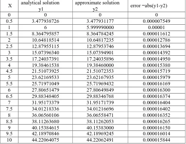
7. Numerical results

In the section, we have solved two problems about Fredholm integral equation of second kind. For the numerical problem, the analytical solution y1has been known in advance, therefore we test the accuracy of the obtained solutions by computing the deviation: error = absolute(y1-y2), where y2 is the numerical solution.

The computer programs which we have used in this work are coded in MATLAB 2015 .

Example 5. The approximation solution of the Fredholm integral equation

∫

+ +

= 1

0

2 1 } ) ( { )

(x x xt xt dt y

Can be described as :

) ) 1 ( 128

5 ) 1 ( 16

1

) 1 ( 8 1 ) 1 )( 2 1 ( exp(xt)(

) 5 , 1 , , ( ) exp(

4 2 1 3

2 1

2 2 1 2

1 2

1

− −

−

+ − −

− +

+ + =

t x t

x

t x t

x x x x t

k taylor xt

(9)

75 ) 128

5 exp(xt)( )

( ), 16

1 exp(xt)( )

(

), 8

1 exp(xt)( )

( ), 2 1 exp(xt)( )

( ), exp(xt)(

) (

2 1

5 2 1

4

2 1

3 2 1

2 2 1

1

x x

f x x

f

x x

f x x x

f

− =

=

− =

+ =

and

4 5

3 4

2 3

2

1(t)=1,g (t)=(t−1),g (t)=(t−1) ,g (t)=(t−1) ,g (t)=(t−1)

g .

Then the approximate solution of this problem is :

2 1 30768 . 2 69231 . 3

2 x x

y = +

the analytical solution of this problem is :

2

1

26 60 26 96

1 x x

y = +

Numerical and analytical solutions of this problem can be found in Table 1.

Table 1: Results for example 5

X analytical solution y1

approximate solution

y2 error =abs(y1-y2)

0 0 0 0

0.5 3.477938726 3.477931177 0.000007549

1 6 5.999990000 0.00001

1.5 8.364795857 8.364784245 0.000011612

2 10.64818514 10.64817235 0.000012786

2.5 12.87955115 12.87953746 0.000013694

3 15.07396340 15.07394901 0.000014392

3.5 17.24037391 17.24035896 0.000014950

4 19.38461538 19.38460000 0.000015380

4.5 21.51073925 21.51072353 0.000015719

5 23.62169533 23.62167935 0.000015979

5.5 25.71971049 25.71969432 0.000016169

6 27.80651479 27.80649849 0.000016300

6.5 29.88348405 29.88346768 0.000016374

7 31.95173379 31.95171739 0.000016404

7.5 34.01218336 34.01216696 0.000016402

8 36.06560106 36.06558471 0.000016352

8.5 38.11263680 38.11262053 0.000016265

9 40.15384615 40.15383000 0.000016150

9.5 42.18970846 42.18969245 0.000016014

(10)

76

8. Conclusion

In this work, we have introduced a modified numerical method for solving linear

Ferdholm integral equation of second kind : = +

∫

b

a

t y t x k x

f x

y( ) ( )

λ

( , ) ( )dt. This

method is based on Taylor series multiplied by the exponential function of (xt) to approximate the kernel k( tx, ) as a summation of multiplication functions f_n(x) by

) (t

g_n i.e.

∑

=

= N

n

n n xg t f t x k

1

) ( ) ( )

,

( , then use the degenerate kernel idea to solve the

Fredholm integral equation. We have solved the Fredholm integral equation with 0

=

a and b=1,

λ

is a real number, f(x) and k( tx, ) are real continues functions. For future studies, one can extend this method to find a numerical solution of the Fredholm integral equation with a≠0and b≠1. Also, one can use this method for solving Volterra integral equation, Fredholm differential equation and Volterra integro-differential equation.

REFERENCES

1. M.D.Raisinghania, Integral equations and boundary value problems, S.Chand & Company Ltd, India (2007).

2. A.R.Vahidi and I.M.Mokhtari, On the decomposition method for system of linear Fredholm integral equations of second kind, Journal of Applied Mathematical Science, 2(2) (2008) 57-62.

3. E.Babolian and H.S.Goghory, Numerical solution of linear Fredholm fuzzy integral equation of second kind by Adomian method, Journal of Applied Mathematics and Computation, 161(3) (2008) 733-744.

4. G.Hanna and J.Roumeliotis, Collocation and Fredholm integral equation of the first kind, Journal of Inequalities in Pure and Applied Mathematics, 6(5) (2009) 131-142. 5. K.Maleknejad and K.M.Tavassoli, Numerical solution of linear Fredholm and Volterra integral equation of second kind by using Legendre wavelets, Kybernete Journal, 32(10) (2010) 1530-1539.

6. M.C.Debonis and C.Laurita, Numerical treatment of second kind Fredholm integral equations systems on bounded intervals, Journal of Computational and Applied Mathematics, 217(1) (2010) 64-87.

7. R.H.Chan and F.U.Rong, A fast solver for Fredholm equation of the second kind with weakly singular kernel, East-West Journal of Numerical Math., 2(3) (2011) 1-24.

8. S.Kumar and A.L.Sangal, Numerical solution of singular integral equations using cubic spline interpolation, India Journal of Applied Mathematics, 35(3) (2011) 415-421.

9. H.H.Hameed and H.M.Abbas, Taylor series method for solving linear Fredholm integral equation of second kind using MATLAB, Pure and Applied Sciences, 19(1) (2011) 13-24.