Memory-Based Shallow Parsing
Erik F. Tjong Kim Sang [email protected]
CNTS - Language Technology Group University of Antwerp
Universiteitsplein 1 B-2610Wilrijk, Belgium
Editors:James Hammerton, Miles Osborne, Susan Armstrong and Walter Daelemans
Abstract
We present memory-based learning approaches to shallow parsing and apply these to five tasks: base noun phrase identification, arbitrary base phrase recognition, clause detection, noun phrase parsing and full parsing. We use feature selection techniques and system combination methods for improving the performance of the memory-based learner. Our approach is evaluated on standard data sets and the results are compared with that of other systems. This reveals that our approach works well for base phrase identification while its application towards recognizing embedded structures leaves some room for improvement.
Keywords: shallow parsing, memory-based learning, feature selection, system combina-tion
1. Introduction
Memory-based learners classify data based on their similarity to data that they have seen earlier. They have been used for a variety of natural language processing tasks with good results, for example for grapheme-to-phoneme conversion (Hoste et al., 2000), stress assign-ment (Daelemans et al., 1994) and word class tagging (Van Halteren et al., 2001). These natural language processing tasks are classification tasks: they require an assignment of a class to each character or to each word. Shallow parsing is more complicated than that: it requires sequences of words to be grouped together and be classified.
We believe that all natural language tasks can be performed successfully by memory-based learners. Identifying and classifying sequences of words can be converted to a classi-fication taskby using special tag sets, for example the IOB tag set proposed by Ramshaw and Marcus (1995). Parsing requires different processing levels and these can be simulated by cascading several memory-based learners which have been trained on different subtasks (Daelemans, 1995). The idea of using memory-based methods for processing natural lan-guage has recently led to the emergence of a new paradigm: Memory-Based Lanlan-guage Processing (MBLP) to which a special issue of the Journal of Experimental & Theoretical Artificial Intelligence was devoted (Daelemans, 1999).
we will examine are identification of base noun phrases, recognition of phrases of arbitrary types, finding clauses, discovering embedded noun phrases and full parsing. Memory-based learning performs well on natural language tasks that require output that has relatively little structure. In this paper we will investigate whether we can obtain equally good results when it is applied to tasks requiring more complex outputs.
2. Approach
In our approach we will use three techniques. We will use memory-based learning as base classification method for assigning linguistic classes to data. We will attempt to solve a weakness of this approach, disregarding irrelevant features, by using an additional feature selection method. Finally, we will examine the combination of several learners in order to obtain an extra performance boost. This section also contains information about evaluation and system configuration for performing parameter tuning.
2.1 Memory-Based Learning
The basic idea behind memory-based learning is that concepts can be classified by their similarity with previously seen concepts. In a memory-based system, learning amounts to storing the training data items. The strength of such a system lies in its capability to compute the similarity between a new data item and the training data items. The most simple similarity metric is the overlap metric (Daelemans et al., 2000). It compares corresponding features of the data items and adds 1 to a similarity rate when they are different. The similarity between two data items is represented by a number between zero and the number of features,n, in which value zero corresponds with an exact match andn
corresponds with two items which share no feature value. Here is an example:
TRAIN1 man saw the V
TRAIN2 the saw . N
TEST1 boy saw the ?
It contains two training items of a part-of-speech (POS) tagger and one test item for which we want to obtain a POS tag. Each item contains three features: the word that needs to be tagged (saw) and the preceding and the next word. In order to find the best POS tag for the test item, we compare its features with the features of the training data items. The test item shares two features with the first training data item and one with the second. The similarity value for the first training data item (1) is smaller than that of the second (2) and therefore the overlap metric will prefer the first.
The method which we use to assign weights to the features is called Gain Ratio, a normalized variant of information gain (Daelemans et al., 2000). It estimates feature weights by examining the training data and determines for each feature how much information it contributes to the knowledge of the classes of the training data items. The weights are normalized in order to account for features with many different values. The Gain Ratio computation of the weights is summarized in the following formulas:
wi = H
(C)−v∈V
iP(v)×H(C|v)
H(Vi) (1)
H(X) =−
x∈X
P(x)log2P(x) (2)
Here wi is the weight of feature i, C the set of class values and Vi the set of values that
featurei can take. H(C) and H(Vi) are the entropy of the setsC and Vi respectively and
H(C |v) is the entropy of the subset of elements ofC that are associated with valuev of featurei. P(v) is the probability that featureihas valuev. The normalization factorH(Vi)
was introduced to prevent that features with low generalization capacities, like identification codes, would obtain large weights.
The memory-based learning software which we have used in our experiments, TiMBL (Daelemans et al., 2000), contains several algorithms with different parameters. In this paper we have restricted ourselves to using a single algorithm (knearest neighbor classifica-tion) with a constant parameter setting. It would be interesting to evaluate every algorithm with all of its parameters but this would require a lot of extra work. We have changed only one parameter of the nearest neighbor algorithm from its default value: the size of the near-est neighborhood region. The learning algorithm computes the distance between the tnear-est item and the training items. The test item will receive the most frequent classification of the nearest training items (nearest neighborhood size is 1). Daelemans et al. (1999) show that using a larger neighborhood is harmful for classification accuracy for three language tasks but not for noun phrase chunking, a task which is central to this paper. In our experiments we have found that using the three nearest sets of data items leads to a better performance than using only the nearest data items. This increase of the neighborhood size used leads to a form of smoothing which can get rid of the influence of some data inconsistencies and exceptions.
2.2 Feature Selection
A disadvantage of the Gain Ratio metric used in memory-based learning is that it computes a weight for a feature without examining other available features. If features are dependent, this will generally not be reflected in their weights. A feature that contains some information about the classification class on its own, but none when another more informative feature is present will receive a non-zero weight. Features which contain little information about the classification class will receive a small weight but a large number of them might still overrule more important features. These two problems will have a negative influence on the classification accuracy, in particular when there are many features available.
200 220 240 260 280 300 320 340 360 380 400
0 2 4 6 8 10
accuracy
number of random features
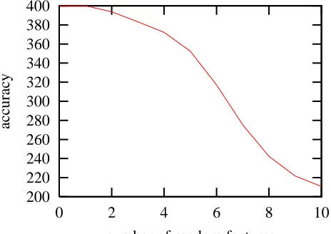
Figure 1: Average number of correct patterns over 1000 runs of a memory-based learner us-ing the Gain Ratio metric for test data containus-ing 400 XOR patterns after addus-ing 0 to 10 random binary features. The system performs perfectly with one random feature but when two or more random features are added, the performance drops to about half for 10 extra features.
we chose is the XOR problem. It contains two binary (0/1) features and a pair of these feature values should be classified as 0 when the values are equal and as 1 when the features are different. We have created training and test data which contained 100 examples of the four possible patterns (0/0/0, 0/1/1, 1/0/1 and (1/1/0). A memory-based learner which uses Gain Ratio was able to correctly classify all 400 patterns in the training data. After this we added ten random binary features to both the training data and the test data and observed the performance. The average results of 1000 runs can be found in Figure 1.
Without extra features the memory-based learner performs perfectly. Adding a random feature does not harm its performance but after adding two the system only gets 394 of the 400 patterns correct on average. The performance drops for every extra added feature to about 211 for 10 extra features which is not much better than randomly guessing the classes. This small experiment shows that Gain Ratio has difficulty with feature sets that contain many irrelevant features. We need an extra method for determining which features are not necessary for obtaining a good performance.
Both the filter and the wrapper method start with a set of features and attempt to find a better set by adding or removing features and evaluating the resulting sets. There are two basic methods for moving through the feature space. Forward sequential selection starts with an empty feature set and evaluates all sets containing one feature. After this it selects the one with the best performance and evaluates all sets with two features of which one is the best single feature. Backward sequential selection starts with all features and evaluates all sets with one feature less. It will selects the one with the best performance and then examines all feature sets which can be derived from this one by removing one feature. Both methods continue adding or removing a feature until they cannot improve the performance. Forward and backward sequential selection are a variant of hill-climbing, a well-known search technique in artificial intelligence. As with hill-climbing, a disadvantage of these methods is that they can get stuckin local optima, in this case a non-optimal feature set which cannot be improved with the method used. In order to minimize the influence of local optima, we use a combination of the two methods when examining feature sets: bidirectional hill-climbing (Caruana and Freitag, 1994). The idea here is to apply both adding a feature and removing a feature at each point in the feature space. This enables the feature selection method to backtrack from nonoptimal choices. In order to keep processing times down we will start with an empty feature list just like in forward sequential selection.
2.3System Combination
When different machine learning systems are applied to the same task, they will make different errors. The combined results of these systems can be used for generating an analysis for the taskthat is usually better than that of any of the participating systems, for example by choosing pattern analyses selected by the majority of the systems. This approach will eliminate errors that made by a minority of the systems. Here is a made-up example: suppose we have five systems, c1 - c5, which assign binary classes to patterns.
Their output for eight patterns, p1 - p8, is as follows:
c1 c2 c3 c4 c5 correct
p1 0 0 0 0 0 0
p2 1 1 1 1 1 1
p3 0 0 0 0 0 0
p4 1 0 1 1 1 1
p5 0 0 1 0 0 0
p6 1 1 1 1 0 1
p7 1 0 0 0 0 0
p8 1 1 1 0 1 1
In this paper we will evaluate different techniques for combining system output, most of which have been put forward by Van Halteren et al. (2001). We use four voting methods and three stacked classifiers. Voting methods assign weights to the output of the individual systems and for each pattern choose the class with the largest accumulated score. The most simple voting method is the one we have used in the preceding example: Majority Voting. It gives all systems the same weight. A more elaborate method is accuracy voting (TotPrecision). It assigns a weight to each system which is equal to the accuracy of the system on some evaluation data.
Some classes might be easier to predict than other classes and for this reason we have also tested two voting methods which use weights based on accuracies for particular class tags. The first is TagPrecision. For each output valuevof systems, it uses a weight which is equal to the precision of that systemsobtained for this valuev. The second method is Precision-Recall. It starts from the same weights as TagPrecision but adds to these the probability that systems producing different output values would have missedv. For example, suppose that there are two systemss1ands2, and that for some data items1 predicts valuev1 while s2 predicts something else. In that case, the probability that s1 is right isprecision(s1, v1)
while the probability that s2 would have missed v1 is 1−recall(s2, v1). Precision-Recall
will assign the weightprecision(s1, v1) + (1−recall(s2, v1)) to the event ofs1 predictingv1.
A stacked classifier is a classifier which processes the results of other classifiers. We have used three variants of stacked classifiers. The first is called TagPair. It examines pairs of values produced by two systems and estimates the probability that a certain output value is associated with the pair. In the case of the two systems s1 and s2 producing two
distinct values v1 and v2, TagPair will examine evaluation data and find that the value
pair is associated with, for example, v1 in 20% of the cases, v2 in 70% and v3 in 10%.
These numbers will be used as weights for the three output values and the one that has accumulated the largest value after examining all value pairs in the pattern, will be selected. Unlike the voting methods, TagPair has the opportunity to choose the correct output tag even if all systems have made an incorrect prediction (for example,v3 in this example).
The other stacked classifier which we have evaluated is the memory-based learner itself. We have tested it in two modes: one in which only the output of the systems was included and one in which we included information about the test item. This extra information was the word that needed to be classified, its part-of-speech (POS) tag and the context (words/POS tags) in which it appeared. The memory-based learner used the same settings as described earlier in this section: it used the Gain Ratio metric and examined a nearest neighborhood of size three.
2.4 Parameter Tuning
In this paper, we will compare different learner set-ups and apply the best one to standard data sets. For example, we will examine different data representations and test different system combination techniques. We should be careful not to tune the system to the test data and therefore we will only use the available training data for finding the best configuration for the learner. This can be done by using 10-fold cross-validation (Weiss and Kulikowski, 1991). The training data will be divided in ten sections of similar size and each section will be processed by a system which has been trained on the other nine. The overall performance on all ten sections will be regarded as the performance of the system.
In our experiments, we will process the data twice. First we will let the learner generate a classification of the data. After this the learner will process the data another time, this time while including the classifications found earlier for the context of a data item. While working with n-fold cross-validation, we should be careful that information from a test part is not accidentally used in its training part. In the first processing phase we will generate classes for the first section while using the other nine sections. Thus information about the classes in, for example, section two is encoded in the classes produced in section one. If in the second phase we use the classifications of the first section while processing section two, we are analyzing a section while having access to (indirect) information about the classes in the data. Information about the classes in section two might leakto this process via the training data, something which is undesired.
There are two ways for preventing this form of information leaking. Both concern being more strict when it comes to creating the training data of the second system. In a cascaded 10-fold cross-validation experiment, the second phase training data for section x must be constructed without using this section. This means that instead of running one 10-fold cross-validation experiment with the first system, we need to run ten 9-fold cross-validation experiments in order to obtain correct training data for the ten sections in the second system. Section one will be trained with the 9-fold cross-validation results from sections 2-10, section 2 with 1 and 3-10 and so on. If at any time we need to add a third phase to the cascade of systems, we need to run 8-fold cross-validation experiments with the first system and 9-fold cross-validation experiments with the second. For extra systems the number of extra runs increases and the amount of available training data for the first system decreases.
Here is an example to illustrate the two methods: suppose a word in the sixth section in the second phase of a ten-fold cross-validation experiment in chunking is represented by the following eight features:
wi−1 wi wi+1 pi−1 pi pi+1 ci−1 ci+1
The goal is to find a chunktag for wordwi. The word featureswi,wi−1 andwi+1represent,
the word itself, the preceding word and the next word, respectively. The POS tag features
pi, pi−1 and pi+1 contain the POS tags of the three words. The two chunkfeatures ci−1
and ci+1 hold the chunktag of the preceding and the next word. The word and POS tag
information have been taken from the training data. In the first method, the two chunk features are computed by a preceding phase. If this item is part of the training data for section x,ci−1andci+1were generated by a nine-fold cross-validation experiment which uses
all sections except section x. This means that the two chunkfeatures have been generated by training with all sections except 6 and x. If the item is part of the test data, then the chunkfeatures are computed by a ten-fold cross-validation experiment (training with sections 1-5 and 7-10). The second method generates chunkfeatures for the test data in the same way but for training data it takesci−1andci+1from the training data, thus preventing
that they contain implicit information about the test sections.1 2.5 Evaluation
We will compare the results of a shallow parser with an available hand-parsed corpus. For this purpose we will use the precision and recall of the phrases in the results. Precision is the percentage of phrases found by the learner that are correct according to the corpus. Recall is the percentage of corpus phrases found by the learner. It is easier to optimize a system configuration based on one evaluation score and therefore we combine precision and recall in the Fβ rate (Van Rijsbergen, 1975):
Fβ = (β
2+ 1)∗precision∗recall
β2∗precision+recall (3)
β can be used for giving precision a larger (β >1) or smaller (β <1) weight than recall. We do not have a preference for one or the other and therefore we use β=1. In previous workon shallow parsing, often a word-related accuracy rate is used as evaluation criterion. We do not believe that this is a good method for evaluating results of phrase detection algorithms. Accuracy rates assign positive values to correctly identified non-phrase words and to partially identified phrases. Furthermore they will produce different numbers for the same analysis based on the data representation used. For these reasons, the relation between accuracy rates and Fβ rates is poor and preference should be given to using the latter.
Accuracy rates have one advantage over Fβ rates: standard statistical tests can be used for determining if the difference between two accuracy rates is significant. Accuracy is a relatively simple function correct/processed where processed is the number of items that have been processed and correct is the number of items that received the correct class.
Unfortunately, Fβ=1 is more complex: after some arithmetic we get 2∗correct/(f ound+ corpus) where f oundis the number of phrases found by the learner,correct the number of phrases found that were correct andcorpus the number of phrases in the corpus according to some gold standard. The value of thecorpusvariable is an upper bound on the variable
correct. The complexity of the Fβ=1computation makes it hard to apply standard statistical
tests to Fβ=1 rates.
Yeh (2000) offers a method for computing significance values for Fβ=1rate comparisons:
by using computationally-intensive randomization tests. His approach requires test data classifications for all systems that need to the compared. Usually we only have access to the test data classifications of our own system and therefore we have used a variant of these randomization tests presented: bootstrap resampling (Noreen, 1989). The basic idea of this approach is to regard the test data classifications as a population of cases. A random sample of this population can be created by arbitrarily choosing cases with replacement. We can create many random samples of the same size as the test data and compute an average Fβ=1
rate over the samples and a standard deviation for this average. These statistical measures can be used for deciding if the performance of another system is significantly different from our system. Since we do not know if the performance of our system is distributed according to a normal distribution, we will determine significance boundaries in such a way that 5% of the samples evaluate worse (or better) than the chosen boundary.
3. Chunking
In this section we will apply a memory-based learner to chunking, identifying base phrases. The section starts with a some background information on this task. After this we will present the results of our experiments with base noun phrase identification and our work targeted at finding base phrases of arbitrary types.
3.1 Task Overview
A text chunker divides sentences in phrases which consist of a sequence of consecutive words which are syntactically related. The phrases are nonoverlapping and nonrecursive. In the beginning of the nineties, Abney (1991) suggested to use chunking as a preprocessing step of a parser. Ten years later, most statistical parsers contained a chunking phase (for example Ratnaparkhi (1998)). In this study, we will divide chunking in two subtasks: finding only noun phrases and identifying arbitrary chunks.
Machine learning approaches towards noun phrase chunking started with work by Church (1988) who used bracket frequencies associated with POS tags for finding noun phrase boundaries in text. In an influential paper about chunking, Ramshaw and Marcus (1995) show that chunking can be regarded as a tagging task. Even more importantly, the authors propose a training and test data set that are still being used for comparing different text chunking methods. These data sets were extracted from the Wall Street Journal part of the Penn TreebankII corpus (Marcus et al., 1993). Sections 15-18 are used as training data and section 20 as test data.2 In principle, the noun phrase chunks present in the material are noun phrases that do not include other noun phrases, with initial material (determiners,
adjectives, etc.) up to the head but without postmodifying phrases (prepositional phrases or clauses) (Ramshaw and Marcus, 1995).
The noun phrase chunking data produced by Ramshaw and Marcus (1995) contains a couple of nontrivial features. First, unlike in the Penn Treebank, possessives between two noun phrases have been attached to the second noun phrase rather than the first. An example in which round brackets mark chunk boundaries: ( Nigel Lawson ) (’s restated commitment ): the possessive’shas been moved fromNigel Lawsontorestated commitment. Second, Treebankannotation may result in nonexpected noun phrase annotations: British Chancellor of ( the Exchequer ) Nigel Lawson in which only one noun chunkhas been marked. The problem here is that neither British Chancellor nor Nigel Lawson has been annotated as separate noun phrases in the Treebank. BothBritish ... ExchequerandBritish ... Lawson are annotated as noun phrases in the Treebankbut these phrases could not be used as noun chunks because they contain the smaller noun phrasethe Exchequer.
Ramshaw and Marcus (1995) proposed to encode chunks with tags: I for words that are inside a noun chunkand O for words that are outside a chunk. In case one noun phrase immediately follows another one, they use the tag B for the first word of the second phrase in order to show that a new phrase starts there. With the three tags I, O and B any chunkstructure can be encoded. This representation has two advantages. First, it enables trainable POS taggers to be used as chunkers by simply changing their training data. Second, it minimizes consistency errors which appear with the bracket representation where open and close brackets generated by the learner may not be balanced. Here is an example sentence first with noun phrases encoded by pairs of brackets and then with the Ramshaw and Marcus IOB representation:
In ( early trading ) in ( Hong Kong ) ( Monday ) , ( gold ) was quoted at ( $ 366.50 ) ( an ounce ) .
InO earlyI tradingI inO HongI KongI MondayB ,O goldI wasO quotedO atO $I 366.50I anB ounceI .O
Tjong Kim Sang and Veenstra (1999) presents three variants on the Ramshaw and Marcus representation and shows that the bracket representation can also be regarded as a tagging representation with two streams of brackets. They named the variants IOB2, IOE1 and IOE2 and used IOB1 as name for the Ramshaw and Marcus representation. IOB2 was the same as IOB1 but now every chunk-initial word receives tag B. IOE1 differs from IOB1 in the fact that rather than the tag B, a tag E is used for the final word of a noun chunkwhich is immediately followed by another chunk. IOE2 is a variant of IOE1 in which each final word of a noun phrase is tagged with E. The bracket representations use open brackets for phrase-initial words, close brackets for phrase-final words and a period for all other words. Table 1 contains example tag sequences for all six tag sequences for the example sentence. The representation variants are interesting because a learner will make different errors when trained with data encoded in a different representation. This means that we can train one learner with five3 data representations and obtain five different analyses of the
data which we can combine with system combination techniques. Thus the different data
IOB1 O I I O I I B O I O O O I I B I O
IOB2 O B I O B I B O B O O O B I B I O
IOE1 O I I O I E I O I O O O I E I I O
IOE2 O I E O I E E O E O O O I E I E O
O . [ . . [ . [ . [ . . . [ . [ . .
C . . ] . . ] ] . ] . . . . ] . ] .
Table 1: The chunktag sequences for the example sentence In early trading in Hong Kong Monday , gold was quoted at$366.50an ounce . for six different tagging formats. The Itag has been used for words inside a chunk,Ofor words outside a chunk, B and[for chunk-initial words andE,]for chunk-final words and periods for words that are neither chunk-initial nor chunk-final.
representations may enable us to improve the performance of the chunker. The data rep-resentations can be used both for noun phrase chunking and for arbitrary chunking. In the latter task, more than one chunk type exists so the tags need to be expanded with type-specific suffixes. For example: B-VP, I-VP, E-VP, [-VP and ]-VP.
The arbitrary chunking task was more difficult to design because many interesting phrase types often contain parts which belong to other phrases (Tjong Kim Sang and Buchholz, 2000). For example, verb phrases may contain noun phrases and prepositional phrases often include a noun phrase. Furthermore, noun phrases may contain quantitative or adjective phrases which may prevent them from being identified as noun chunks. The noun, verb and prepositional phrases should be included and therefore the following measures have been taken when constructing the data for the arbitrary chunking task: First, a couple of phrase types, for example quantifier phrases and adjective phrases, have been removed from places where they prevented the identification of noun phrases. This made possible annotating more phrases as noun chunks. Second, some phrase types in the annotated data, for example verb phrases and prepositional phrases, lackmaterial that has already been included in a phrase of another type. Third, adjacent verb clusters have been put in one flat verb phrase unlike in the Treebank where often each verb starts a new phrase. And fourth, adverbial phrase boundaries have been removed from adjective phrases and verb phrases to allow all material to be included in the mother phrase.
This chunkdefinition scheme will generate data in which most of the tokens have been assigned to a chunkof some type. The odd tokens that fall out are usually punctuation signs. This chunkscheme has been used for generating training and test data for the CoNLL-2000 shared task(Tjong Kim Sang and Buchholz, 2000). The data contains the same segments of the Wall Street Journal part of the Penn Treebankas the noun phrase data of Ramshaw and Marcus (1995): sections 15-18 as training data and section 20 as test data.4 We will use these data sets in our arbitrary chunking experiments.
The training and the test data contain two types of features: words and POS tags. The words have been taken from the Penn Treebank. The POS tags of the Treebank have been manually checked and therefore they should not be used in the chunking data. In future
applications, the chunking process will be applied to a text with POS tags that have been generated automatically. These POS tags will contain errors and therefore the performance of the chunker will be worse than when applied to a Treebank text with manually checked POS tags. If we want to obtain realistic performance rates, we should workwith automat-ically generated POS tags in our shallow parsing experiment. Conform with earlier work like that of Ramshaw and Marcus (1995), we have used POS tags that were generated by the Brill tagger (Brill, 1994).
3.2 Noun Phrase Recognition
We will use a memory-based learner to find noun phrase chunks in text. In order to determine the best configuration for the learner, we will test different system configurations on the standard training data sets put forward by Ramshaw and Marcus (1995). We will evaluate different feature sets for representing words. Additionally, we will use the five data representations for generating different system results and use system combination techniques for combining these results.
In our experiments we will represent words as sets of words and POS tags. These sets contain the word itself, its part-of-speech (POS) tag and a left and right context of a maximum of four words and POS tags on each side, 18 features in total. We have explained in Section 2.2 that memory-based learners equipped with the Gain Ratio metric have difficulty in dealing with irrelevant features. Therefore we will use a feature selection method, bi-directional hill-climbing starting with zero features, for finding the best subset of the 18 features for each different data representation.
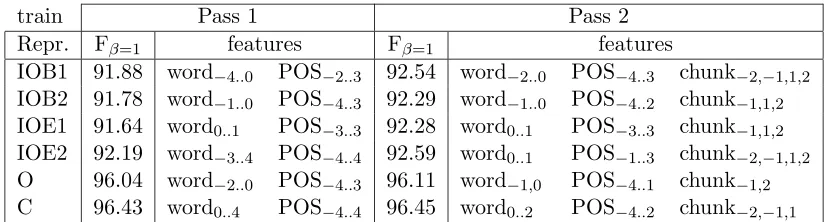
The memory-based learner will make two passes over the data. First, it will attempt to predict the noun phrases in the data as well as possible. After this it will use the output of this first pass as information about the noun phrases in the immediate context of the current word. This means that the second pass has access to the 18 features of the first pass plus the chunktags of the two words immediately in front of the current word and the chunktags of the two words immediately following the current word. This cascaded approach was chosen because it was useful for improving overall performance in our earlier work(Tjong Kim Sang and Veenstra, 1999). We omitted the chunktag for the current word because including it gave a negative bias to the chunker performance. Gain Ratio would correctly identify it as a feature which contained a lot of information about the output class and the weight it assigned to it would make it hard for the other features to influence the output class at all (Tjong Kim Sang and Veenstra, 1999).5
We performed a cascaded feature search while using five different data representations on the training data of Ramshaw and Marcus (1995) in a 10-fold cross-validation approach. We prevented information leaking in the second phase conform Section 2.4 by using the estimated chunktags for test data and using the corpus tags in the training data. In this way we made sure that when the test data consisted of section x, no information about section x was available in the training data. The results of the 10-fold cross-validation
train Pass 1 Pass 2
Repr. Fβ=1 features Fβ=1 features
IOB1 91.88 word−4..0 POS−2..3 92.54 word−2..0 POS−4..3 chunk−2,−1,1,2
IOB2 91.78 word−1..0 POS−4..3 92.29 word−1..0 POS−4..2 chunk−1,1,2
IOE1 91.64 word0..1 POS−3..3 92.28 word0..1 POS−3..3 chunk−1,1,2
IOE2 92.19 word−3..4 POS−4..4 92.59 word0..1 POS−1..3 chunk−2,−1,1,2
O 96.04 word−2..0 POS−4..3 96.11 word−1,0 POS−4..1 chunk−1,2
C 96.43 word0..4 POS−4..4 96.45 word0..2 POS−4..2 chunk−2,−1,1
Table 2: Best Fβ=1 found for six data representations in two passes while using a
bi-directional hill-climbing feature search algorithm in a 10-fold cross-validation pro-cess applied to the training data for the noun phrase chunking task. Note that the rates obtained for the O (open bracket) and C (close bracket) representations are for phrase starts and phrase ends respectively and thus higher than for the first four which evaluate complete phrase identification.
experiments can be found in Table 2. In the best feature sets of the first pass most of the nine POS tag features are used (almost eight on average) but interestingly enough only a few of the word features (just over four on average). The best sets for the second pass use fewer POS tag features (under seven), fewer word tags (just over two) and most of the chunkfeatures (about three). The table shows that a wide context is more important for the POS features than for the chunkfeatures and less important for the word features.
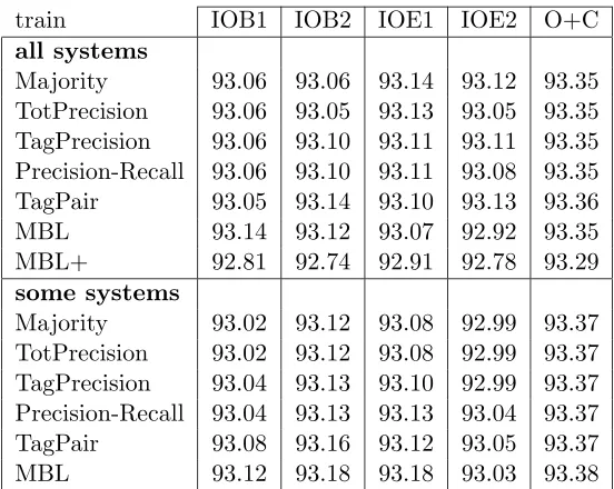
Our motive for processing six representations rather than one was to obtain different results which we could combine in order to improve performance. System combination can be seen as a second cascade behind passes one and two. For reasons mentioned in Section 2.4, adding a second cascade in a 10-fold cross-validation experiment requires taking extra care to prevent information leaking from a training data at one level to the training data of the next level. We have taken care of this problem by preparing the training data of the combination techniques with 9-fold cross-validation runs which were independent of the 10-fold cross-validation experiments used for generating the test data. For example, the test data for the first section was generated by training with sections 2-10 twice, first without information about context chunktags and then with the perfect information of the context chunktags. The training data was generated with a 9-fold cross-validation process on sections 2-10, also first without context chunktags and then with perfect context chunk tags. By working this way it was impossible for information about the first section to enter the training data of the combination processes.
train IOB1 IOB2 IOE1 IOE2 O+C all systems
Majority 93.06 93.06 93.14 93.12 93.35
TotPrecision 93.06 93.05 93.13 93.05 93.35
TagPrecision 93.06 93.10 93.11 93.11 93.35
Precision-Recall 93.06 93.10 93.11 93.08 93.35
TagPair 93.05 93.14 93.10 93.13 93.36
MBL 93.14 93.12 93.07 92.92 93.35
MBL+ 92.81 92.74 92.91 92.78 93.29
some systems
Majority 93.02 93.12 93.08 92.99 93.37
TotPrecision 93.02 93.12 93.08 92.99 93.37
TagPrecision 93.04 93.13 93.10 92.99 93.37
Precision-Recall 93.04 93.13 93.13 93.04 93.37
TagPair 93.08 93.16 93.12 93.05 93.37
MBL 93.12 93.18 93.18 93.03 93.38
Table 3: Fβ=1 rates obtained on 10-fold cross-validation experiments on the noun phrase
chunking data while combining results obtained with five different data representa-tions. All five representations have been tested and best rates have been obtained while using the the combined bracket representation O+C. All combination re-sults are better than any result of the individual systems (92.59, see Table 2) and generally combing five systems led to better results than when only three or four were used. The best results have been obtained with a stacked memory-based classifier that used all system results except those generated with IOE1. However, the performance differences are small.
these by removing all brackets which cannot be matched with the closest candidate. For example, if we have a structure like ( a ( b c ) d ) then the first bracket will be removed because it cannot be matched with the second bracket. The second and third will be kept because they match. Finally, the fourth will be removed because it cannot be matched with the third. We obtain the balanced structurea ( b c ) dwhich can trivially be converted to the four IO formats.
the best results (obtained with context feature current POS tag). System combination im-proved performance: the worst result of the combination techniques is still better than the best result of the individual systems. The differences between the combination techniques are small. Furthermore, system combination with the four IO data representations leads to similar results but the combined bracket representation consistently obtains higher Fβ=1
rates. It should be noted though that while combination of the data with the IO represen-tations leads to similar precision and recall figures, O+C obtains its higher Fβ=1 rates with
high precision rates and lower recall rates.
Since the performance differences between the combination techniques displayed in Table 3 are small, we are relatively free in selecting a technique for further processing. We chose Majority Voting because it is the simplest of the combination techniques that were tested since it does not require extra combinator training data like the other techniques. It does seem reasonable to use the O+C representation during the combination process because the best results have been obtained with this representation. We will restrict ourselves to a few systems rather than combining all because Majority Vote in combination with the O+C representation obtained a slightly higher Fβ=1 rate that way. The best rate was obtained
while using only the systems with data representations IOB1, IOE2 and O+C so we restrict ourselves to these three. This leaves us with the following processing scheme:
1. Process the test data with a memory-based model generated from the training data. Use the features shown in Table 2 (Pass 1) and generate output data streams while using the representations IOB1, IOE2, O and C.
2. Perform a second pass over the test data with another memory-based model obtained from the training data. Again use the features shown in Table 2 (Pass 2). In the test data, use the estimated chunktags from the previous run as chunktag features and in the training data use the corpus chunktags as chunkfeatures. Perform these passes four times, once for each of the data representations IOB1, IOE2, O and C.
3. Convert the output for the data representations IOB1 and IOE2 to the O and the C format.
4. Combine the three O data streams (IOB1, IOE2 and O) with Majority Voting and do the same for the three C data streams (IOB1, IOE2 and C).
5. Remove brackets from the resulting O and C data streams which cannot be matched with other brackets. The balanced bracket structure is the analysis of the test data that is the output of the complete system.
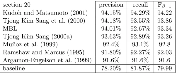
We have applied this procedure to the data sets of Ramshaw and Marcus (1995): sections 15-18 of the Wall Street Journal part of the Penn Treebank(Marcus et al., 1993) as training data and section 20 of the same corpus as test data. The system obtained a Fβ=1 rate of
93.34 (precision 94.01% and recall 92.67%). This is a modest improvement of our earlier work(Tjong Kim Sang, 2000a) in which we did not use feature selection and where we obtained an Fβ=1rate of 93.26. In order to estimate significance thresholds, we have applied
of sentences in each population was the same as in the test corpus. The average Fβ=1 of
the 10,000 populations was 93.33 with a standard deviation of 0.24. For 5 percent of the populations, the Fβ=1 rate was equal to or lower than 92.93 and for another 5 percent it
was equal to or higher than 93.73. Since 93.26 is between the two significance boundaries, our current system does not perform significantly better than the previous version without feature selection.
3.3 Arbitrary Phrase Identification
Our workwith chunks of arbitrary types6 is similar to that with noun phrase chunks apart
from two facts. First, we refrained from using feature selection methods. Applying these methods did not gain us much for noun phrase chunking but they required a lot of extra computational work. Therefore we went back to using a fixed set of features in these experiments. The context size we used here was four left and four right for words and POS tags in the first pass over the data, and three left and three right for words and POS tags, and two left and two right without the focus for chunktags in the second pass. This means that both first and second pass use 18 features. The second pass has only been used for the four IO data representations. Table 2 shows that the second pass improved the performance of the first pass only by a small margin for the two bracket representations O and C.
The second difference between this study and the one for noun phrase chunks originates from the fact that apart from chunkboundaries, we need to find chunktypes as well. We can approach this taskin two ways. First, we could train the learner to identify both chunkboundaries and chunktypes at the same time. We have called this approach the Single-Phase Approach. Second, we could split the taskand train a learner to identify all chunkboundaries and feed its output to another classifier which identifies the types of the chunks (Double-Phase Approach). A computationally-intensive approach would be to develop learners for each different chunktype. They could identify chunks independently of each other and words assigned to more than one chunkcould be disambiguated by choosing the chunktype that occurs most frequently in the training data (N-Phase Approach). Since we did not know in advance which of these three processing strategies would generate the best results, we have evaluated all three.
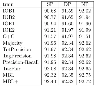
In order to find the best processing strategy and the best combination technique, we have performed several 10-fold cross-validation experiments on the training data. We have processed this data for each processing strategy and in each of the six data representations earlier used for noun phrase chunking. After this we have used the seven combination techniques presented in Section 2.3 for combining these. The results can be found in Table 4. Of the three processing strategies, the N-Phase Approach generally performed best with Double-Phase being second best and Single-Phase performing worst. Again, system combination improved all individual results. There were only small differences between the seven combination techniques when compared for the same processing approach. The only exception were the two stacked MBL classifiers applied to the Single-Phase Approach results. They did about 0.3 Fβ=1rate better than most of the other combination techniques.
train SP DP NP
IOB1 90.68 91.59 92.02
IOB2 90.77 91.65 91.94
IOE1 90.94 91.60 91.90
IOE2 91.21 91.97 91.99
O+C 91.57 91.97 91.51
Majority 91.96 92.34 92.62
TotPrecision 91.97 92.34 92.62
TagPrecision 91.98 92.34 92.62
Precision-Recall 91.96 92.34 92.62
TagPair 92.08 92.34 92.65
MBL 92.32 92.35 92.75
MBL+ 92.40 92.32 92.72
Table 4: Fβ=1 rates obtained for the three processing strategies, Single-Phase Approach
(SP), Double-Phase Approach (DP) and N-Phase approach (NP), when applied to the training data of the CoNLL-2000 shared task(arbitrary chunking) while using five different data representations and seven system combination techniques. In all cases, system combination led to performances that were better than the individual system results. The computationally-intensive N-Phase Approach does better than the other two.
The best result was generated with the N-Phase Approach in combination with a stacked memory-based classifier (MBL, 92.76). A bootstrap resampling test with 8000 random populations generated the 90% significance interval 92.60-92.90 which means that this result is significantly better than any Single-Phase or Double-Phase result. However, the N-Phase approach has a big computing overhead: the number of passes over the data is at least N times the number of representations. Therefore, we have chosen the Double-Phase Approach combined with Majority Voting for our further work. This approach combines a reasonable performance with computational efficiency. The Single-Phase Approach is potentially faster but its performance is worse unless we use a stacked classifier which requires extra combinator training data.
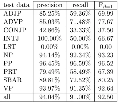
When we applied the Double-Phase Approach combined with Majority Voting to the CoNLL-2000 data sets, we obtained an Fβ=1 rate of 92.50 (precision 94.04% and recall
91.00%). An overview of the performance rates of the different chunktypes can be found in Table 5. Our system does well for the three most frequently occurring chunktypes, noun phrases, prepositional phrases and verb phrases, and less well for the other seven. The chunktype UCP which occurred in the training data, was not present in the test data. With this result, our memory-based arbitrary chunker finished third of eleven participants in the CoNLL-2000 shared task. The two systems that performed better were Support Vector Machines (Kudoh and Matsumoto, 2000, Fβ=1=93.48) and Weighted Probability
test data precision recall Fβ=1
ADJP 85.25% 59.36% 69.99
ADVP 85.03% 71.48% 77.67
CONJP 42.86% 33.33% 37.50
INTJ 100.00% 50.00% 66.67
LST 0.00% 0.00% 0.00
NP 94.14% 92.34% 93.23
PP 96.45% 96.59% 96.52
PRT 79.49% 58.49% 67.39
SBAR 89.81% 72.52% 80.25
VP 93.97% 91.35% 92.64
all 94.04% 91.00% 92.50
Table 5: The results per chunktype of processing the test data with the Double Pass Approach and Majority Voting. Although the data is formatted differently than the noun phrase chunking data, the NP Fβ=1 rate here (93.23) is close to that of
our NP chunking Fβ=1 rate (93.34).
4. Parsing
In this section we will examine the application of memory-based shallow parsing to gener-ating embedded structures. We will examine three tasks: clause identification, noun phrase parsing and full parsing. Whenever possible, we will use the methods that we have applied to chunking in the previous section.
4.1 Clause Identification
In clause identification the goal is to divide sentences in clauses which typically contain a subject and a predicate. We have used the clause data of the CoNLL-2001 shared task (Tjong Kim Sang and D´ejean, 2001) which was derived from the Wall Street Journal Part of the Penn Treebank(Marcus et al., 1993). Here is an example sentence from the Treebank, with all information but words and clause brackets omitted:
(S Coach them in
(S–NOM handling complaints) (SBAR–PRP so that
(S they can resolve problems immediately) )
. )
these data sets contained words and part-of-speech tags which were generated by the Brill tagger (Brill, 1994). Additionally they contained chunktags which were computed by the arbitrary chunking method we discussed in the previous section.
We have approached identifying clauses in the following way:7 first we evaluated different
memory-based learners for predicting the positions of open clause brackets and close clause brackets, regardless of their level of embedding. The two resulting bracket streams will be inconsistent and in order to solve this we have developed a list of rules which change a possibly inconsistent set of brackets to a balanced structure. The evaluation of the learners and the development of the balancing rules will be done with 10-fold cross-validation of the CoNLL-2001 training data. Information leaking is prevented by using corpus clause tags as context features in the training data of cascaded learners rather than clause tags computed in a previous learning phase. The best learner configurations and balancing rules found will be applied to the data for the clause identification shared task.
Like in our noun phrase chunking work, we have tested memory-based learners with different sets of features. At the time we performed these experiments, we did not have access to feature selection methods and therefore we have only evaluated a few fixed feature configurations:
1. words only (w) 2. POS tags only (p) 3. chunktags only (c) 4. words and POS tags (wp) 5. words and chunktags (wc) 6. POS tags and clause tags (pc)
7. words, POS tags and chunktags (wpc)
All feature groups were tested with four context sizes: no context information or informa-tion about a symmetrical window of one, two or three words. Like in our chunking work, we want to checkif an improved performance can be obtained by using system combina-tion. However, since we attempt to predict brackets at all levels in one step, we cannot use the five data representations here. Instead we have evaluated combination of some of the feature configurations mentioned above: a majority vote of the three using a sin-gle type of information (1+2+3), a majority vote of the three using pairs of information (4+5+6) and a majority vote of the previous two and the one using three types of informa-tion (7+(1+2+3)+(4+5+6)). The last one is a combinainforma-tion of three results of which two themselves are combinations of three results.
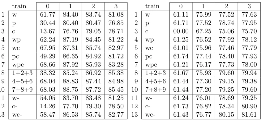
Clauses may contain many words and it is possible that the maximal context used by the learner, three words left and right, is not enough for predicting clause boundaries accurately. However, we cannot make the context size much larger than three because that would make it harder for the learner to generalize. We have tried to deal with this problem by evaluating another set of features which contain summaries of sentences rather than every word. Since we have chunkinformation of the sentences available, we can compress them by removing all words from each chunkexcept the main one, the head word. The head
train 0 1 2 3 train 0 1 2 3
1 w 61.77 84.40 83.74 81.08 1 w 61.11 75.99 77.52 77.63
2 p 30.44 80.40 80.47 76.85 2 p 61.71 77.52 78.74 77.95
3 c 13.67 76.76 79.05 78.71 3 c 00.00 67.25 75.06 75.70
4 wp 62.24 87.19 84.45 81.22 4 wp 61.25 76.52 77.92 78.12
5 wc 67.95 87.31 85.74 82.97 5 wc 61.01 75.96 77.46 77.79
6 pc 49.29 86.65 84.92 81.72 6 pc 61.74 77.44 78.40 77.93
7 wpc 68.66 87.92 85.93 83.28 7 wpc 61.21 76.17 77.73 78.00
8 1+2+3 38.32 85.24 86.92 85.38 8 1+2+3 61.67 75.93 79.60 79.94
9 4+5+6 68.04 88.83 87.44 84.98 9 4+5+6 61.44 77.30 79.15 79.38
10 7+8+9 68.03 88.75 87.72 85.45 10 7+8+9 61.44 77.20 79.25 79.60
11 w- 54.05 83.70 83.48 81.25 11 w- 61.24 76.01 78.69 79.25
12 c- 14.26 77.70 79.30 78.50 12 c- 61.73 76.82 78.34 80.90
13 wc- 58.47 86.53 85.74 82.77 13 wc- 61.43 76.77 80.15 81.61
Table 6: Fβ=1 rates obtained in 10-fold cross-validation experiments with the training data
while predicting open clause brackets (left) and close clause brackets (right). We used different combinations of information (w: words, p: POS tags and c: chunk tags) and different context sizes (0-3). The best results for open brackets have been obtained with a majority vote of three information pairs while using context size 1 (row 9) For close clause brackets best results were obtained with words and POS tags after compressing the chunks and while using context size 3 (row 13).
words can be generated by a set of rules put forward by Magerman (1995) and modified by Collins (1999).8 After removing the nonhead words from each chunk, we can replace the POS tag of the remaining word with the chunktag and thus obtain data with words and chunktags only (words outside of a chunkkeep their POS tag). Again we have evaluated sets of features which hold a single type of information, words (w–) or chunktags (c–), or pairs of information, words and chunktags (wc–).
We have evaluated the twelve groups of feature sets while predicting the clause open and clause close brackets. The results can be found in Table 6. The learner performed best while predicting open clause brackets with information about the words immediately next to the current word (column 1). When more information was available, its performance dropped slightly. Of the different feature sets tested, the majority vote of sets that used pairs of information performed best (column 1, row 9). The classifiers that generated close brackets improved whenever extra context information became available. The best performance was reached while using a pair of words and chunktags in the summarized format (column 3, row 13). We have performed an extra experiment to test if the system improved when using four context words rather than three. With words and chunktags in the summarized format the system obtained Fβ=1=81.72 for context size four compared
with 81.61 for context size three. This increase is small so we have chosen context size three for our further experiments.
With the streams of open and close brackets, we attempted to generate balanced clause structures by modifying the data streams with a set of heuristic rules. In these rules we gave more confidence to the open bracket predictions since, as can be seen in Table 6 the system performs better in predicting open brackets than close brackets. After testing different rule sets created by hand and evaluating these on the available training data, we decided on using the following rule set:
1. Assume that exactly one clause starts at each clause start position.
2. Assume that exactly one clause ends at each clause end position but
3. ignore all clause end positions when currently no clause is open, and
4. ignore all clause ends at non-sentence-final positions which attempt to close a clause started at the first word of the sentence.
5. If clauses are opened but not closed at the end of the sentence then close them at the penultimate word of the sentence.
These rules were able to generate complete and consistent embedded clause structures for the output that the system generated for the training data of the CoNLL-2001 shared task. The rules have one main defect: they are incapable of predicting that two or more clauses start at the same position. This will make it impossible for the system to detect such clause start but unfortunately, according to our rule set evaluation, adding recognition facilities for such multiple clause start would have a negative influence on overall performance levels. This set of rules obtained a clause Fβ=1 of 71.34 on the training data of this taskwhen
applied to the best results for open and close brackets. The rules did not change the open bracket positions and on average the changes they made to the close bracket positions were an improvement (Fβ=1 = 84.11 compared to 81.61).
An argument which could be made is that since open bracket prediction is more accurate than close bracket prediction, one could use the information of the open bracket positions when predicting clause close brackets. We have attempted to do this by repeating the experiment with the best configuration for close brackets (wc– with context size 3) while adding a feature which stated at which clause level the current word was, according to earlier open and close brackets. This approach improved the Fβ=1 rate of the close bracket
predictor from 81.61 to 83.50. However, after applying the balancing rules to the open brackets and the improved close brackets, we only got a clause Fβ=1 of 71.39, a minimal
improvement over the previous 71.34. It seems that the extra performance gain obtained in the close bracket predictor was obtained by solving problems which could already be solved by the balancing rules.
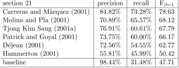
We applied the balancing rules together with an open bracket predictor using a combina-tion of pairs of feature types (context size 1) and a close bracket predictor using summarized pairs of words and chunktags (context size 3) to the data files of the CoNLL-2001 shared task. Our clause identification method obtained an Fβ=1 rate of 67.79 for identifying
and ours is that they use a larger number of features, methods for predicting multiple co-occurring clause starts and a more advanced statistical model for combining brackets to clauses.
In a post-conference study, we have attempted to estimate more precisely the cause of the performance difference between our method an the boosted decision trees used by Carreras and M`arquez (2001). Our hypothesis was that not only the choice of system made a difference, but also the choice of features. For this purpose, Carreras and M`arques kindly repeated an experiment in predicting open brackets but this time while using our feature set: pairs of information using a window of one word left and one right, while results were combined with majority voting (Table 6, left, row 9, column 1). The experiment was performed while testing on the CoNLL-2001 development data set. Originally the memory-based learner obtained Fβ=1 = 89.80 on this data set while their boosted decision
tree approach reached 93.89. However, while using the memory-based feature set, the performance of the decision trees dropped to 91.32. When both systems use the same features, the boosted decision trees outperform the memory-based learner. But it is able to perform better with its own feature set. Our hypothesis was correct: the performance difference between the two approaches was both caused by choice of the learner and the choice of the feature set.
The next obvious question is whether the memory-based system would perform better with the feature set of the boosted decision trees. Providing an answer to this question was nontrivial. The feature set consisted of thousands of binary features which were more than the memory-based learner could handle. After converting the features from binary-valued to multi-valued, there were about 70 features left. At best, the system obtained Fβ=1 =
90.52 with this feature set. Since we feared that still the number of features was too large for the system to handle, we performed a forward sequential selection search process in the feature space starting with zero features. The memory-based learner reached an optimal performance with 13 features at Fβ=1 = 91.82. These results show that there is still room
for improvement for the memory-based learner but that cooperation with a feature selection method will be helpful.
4.2 Noun Phrase Parsing
Noun phrase parsing is similar to noun phrase chunking but this time the goal is to find noun phrases at all levels. This means that just like in the clause identification task we need to be able to recognize embedded phrases. The following example sentence will illustrate this:
In ( early trading ) in ( Hong Kong ) ( Monday ) , ( gold ) was quoted at ( ( $ 366.50 ) ( an ounce ) ) .
We will recover noun phrases at different levels by performing repeated chunking (Tjong Kim Sang, 2000a). We will start with data containing words and part-of-speech tags and identify the base noun phrases in this data with techniques used in our noun phrase chunking work. After this we will replace the phrases that were found by the head words and their tags. This will create a summary of the sentences with words and a mixed data stream of POS tags and chunktags. We can apply our noun phrase chunking techniques to this data one more time and find noun phrases one level above the base level. The compressing and chunking steps will be repeated in order to retrieve phrases at higher levels. The process will stop when no new phrases are found.
The approach described here seems a trivial expansion of our noun phrase chunking work. However, there are some details left to discuss. First, there is the selection of the head word duing the phrase summarization process. At the time we performed these experiments, we did not have access to the Magerman/Collins set of rules for determining head words, and therefore we used a rule created by ourselves: the head word of a noun phrase is the final word of the first noun cluster in the phrase or the final word of the phrase if it does not contain a noun cluster.
The second fact we should mention, is that the data we used contains a different format of noun phrase chunks than the data we previously have worked with. In this task we use the data set which was developed for the noun phrase bracketing shared task of CoNLL-99 (Osborne, 1999). It was extracted from the Wall Street Journal part of the Penn Treebank (Marcus et al., 1993) without extra modifications and this means, for example, that posses-sives between two noun phrases have been attached to the first one unlike in the noun phrase chunking data. This and other differences make that we cannot be sure that the techniques we developed for the other base noun phrase format will workvery well here. Indeed, there is a performance drop in the chunking part of our shallow parser when compared with the chunking work (Fβ=1 of 92.77 compared with 93.34). However, we decided not to put extra
workin searching for a better configuration for our noun phrase chunker and have trained an existing chunker with the data available for this task.
An unforeseen problem occurred when we attempted to use the chunker for identifying noun phrases above the base level. Our chunker output is a majority vote of five systems using different data representations. In our evaluation workwith tuning data (WSJ section 21), we observed that the overall output of the chunker at nonbase levels was worse than the performance of the best individual system (Tjong Kim Sang, 2000a). The reason for this is that the system that used the O+C data representation, outperformed the other four systems by a large margin. Because of this, and probably because the other four systems made similar errors, the errors of the four cancelled some of the correct analyses of the best system and caused the majority vote to be worse than the best individual system. For this reason we have decided to use only the bracket representations when processing noun phrases above base levels.
of the current level and the previous, and those of the current level and the next. At all levels, using the brackets of the current level only proved to be working best or close to best. At the sixth level no new noun phrases were detected. Therefore we decided to use only brackets of one phrase level in the training data for nonbase phrases and stop phrase identification after six levels.
We have applied a noun phrase chunker with fixed symmetrical context sizes to the noun phrase data of the CoNLL-99 shared task(Tjong Kim Sang, 2000a). The chunker generated a majority vote of open and close brackets put forward by five systems, each of which used a different representation of the base noun phrases (IOB1, IOB2, IOE1, IOE2 and O or C). All systems used a window of four left and four right for words and POS tags (18 features) and the four systems using IO representations additionally performed and extra pass with a window of three left and three right for words and POS tags, and a window of two left and two right without the focus tag for chunktags (also 18 features). The output of the chunker was presented to a cascade of six chunkers, each of which consisted of a pair of open and close bracket predictors which were trained with brackets from one of the levels 1 to 6. After each chunkphase the phrases found were replaced by the head word of the phrase and a fixed chunktag.
The system obtained an overall Fβ=1 rate of 83.79 (precision 90.00% and recall 78.38%)
for identifying arbitrary noun phrases.9 It is slightly better than our performance at CoNLL-99 (82.98, obtained without system combination) which was the best of two entries submit-ted for the shared taskat that workshop. The performance of our noun phrase chunker can be regarded as a baseline score for this data set. This score is already quite high: Fβ=1 =
79.70, and it seems that the nonbase level chunkers have not been contributing much to the performance of this shallow parser. Out of curiosity we have also examined how well a full parser does on the taskof identifying arbitrary noun phrases. For this purpose we looked at output data of a parser described by Collins (1999) which was provided with the parser code (WSJ section 23, model 2). The parser obtained Fβ=1 = 89.8 (precision 89.3% and recall
90.4%) for this task. This is a lot better than our shallow parser but we should note that compared with our application, the Collins parser has access to better part-of-speech tags and more training data with more sophisticated annotation rather than only noun phrase boundaries.
4.3Full Parsing
The approach for parsing noun phrases outlined in the previous section can be used for generating parse trees containing phrases of arbitrary phrases as well. In that case we would be using chunking techniques for performing full parsing. The is not a new idea. Ejerhed and Church (1983) present a Swedish grammar which includes noun phrase chunk rules. Abney (1991) describes a chunkparser which consists of two parts: one that finds base chunks and another that attaches the chunks to each other in order to obtain parse trees. Daelemans (1995) suggested to find long-distance dependencies with a cascade of lazy learners among which were constituent identifiers. Ratnaparkhi (1998) built a parser based on a chunker with an additional bottom-up process which determines at what position to start new phrases or to join constituents with earlier ones. With this approach he obtained
state-of-the-art parsing results. Brants (1999) applied a cascade of Markov model chunkers to the taskof parsing German sentences. We have extended our noun phrase parsing techniques to parsing arbitrary phrases (Tjong Kim Sang, 2001b). We will present the main findings of this study here as well.
The standard data sets for testing statistical parsers are different than the ones we used for our earlier workon chunking and shallow parsing. The data sets have been extracted from the Wall Street Journal (WSJ) part of the Penn Treebank(Marcus et al., 1993) as well but they contain different segments. The training data consists of sections 02-21 (39,832 sentences) while section 23 is used as test data (2416 sentences). The data sets consists of words, and part-of-speech tags which have been generated by the part-of-speech tagger described by Ratnaparkhi (1996). In the data the phrase types ADVP and PRT have been collapsed into one category and during evaluation the positions of punctuation signs in the parse tree have been ignored. These adaptations have been done by different authors in order to make it possible to compare the results of their systems with the first study that used these data sets (Magerman, 1995) and all follow-up work.
In our workon arbitrary parsing, we were interested in finding an answer to four ques-tions. In order to obtain these answers, we have performed tests with smaller data sets which were taken from the standard training data for this task: WSJ sections 15-18 as training data and section 20 as test data. The first topic we were interested in, was the influence of context size and size of the examined nearest neighborhood size (parameter k of the memory-based learner) on the performance of the parser. We tookthe noun phrase parser developed in the previous section, lifted its restriction of generating noun phrases only and applied it to this data set while using different context sizes and values for param-eter kfor the classifiers that identified phrases above the base levels. The different types of the chunks were derived by using the Double-Phase Approach for chunking (see Section 3.3). The best configuration we found was a context of two left and two right words and POS tags with kis 1. The nearest neighborhood size is smaller than used in our earlier work(3) and the best context size is smaller than in our noun phrase chunking work(4). However, the best context size we found for this taskis exactly the same as reported by Ratnaparkhi (1998).
The second topic we were interested in was the type of training data that should be used for finding phrases above the base level. In our noun phrase parsing work, we found that the best performance could be obtained by using only data of the current phrase level. This will cause a problems for our parser, since the tree depth may become as large as 31 in our corpus but there will be few training material available for these high level phrases if we use the same training configuration as in our noun phrase parsing work. We have tested two different training configurations to see if we could use more training data for this taskwithout losing performance. With the first of these, using the current, previous and next phrase level, performance was as well (Fβ=1=77.13) as while using only the current
level (77.17). However, when we trained the cascade of chunkers while using brackets of all phrase levels, the performance dropped to 67.49. We have decided to keep on using the current phrase level only in the training data despite its problems with identifying higher level phrases.
![Table 1: The chunk tag sequences for the example sentence In early trading in Hong KongMonday , gold was quoted at $ 366.50 an ounce .for six different tagging formats.The I tag has been used for words inside a chunk, O for words outside a chunk, Band [ for chunk-initial words and E, ] for chunk-final words and periods for wordsthat are neither chunk-initial nor chunk-final.](https://thumb-us.123doks.com/thumbv2/123dok_us/9844770.1970967/11.612.114.497.89.175/sequences-example-sentence-kongmonday-dierent-outside-wordsthat-initial.webp)