Beyond Independent Components: Trees and Clusters
Francis R. Bach [email protected]
Computer Science Division University of California Berkeley, CA 94720, USA
Michael I. Jordan [email protected]
Computer Science Division and Department of Statistics University of California
Berkeley, CA 94720, USA
Editors: Te-Won Lee, Jean-Franc¸ois Cardoso, Erkki Oja and Shun-ichi Amari
Abstract
We present a generalization of independent component analysis (ICA), where instead of looking for a linear transform that makes the data components independent, we look for a transform that makes the data components well fit by a tree-structured graphical model. This tree-dependent component analysis (TCA) provides a tractable and flexible approach to weakening the assumption of independence in ICA. In particular, TCA allows the underlying graph to have multiple connected components, and thus the method is able to find “clusters” of components such that components are dependent within a cluster and independent between clusters. Finally, we make use of a notion of graphical models for time series due to Brillinger (1996) to extend these ideas to the temporal setting. In particular, we are able to fit models that incorporate tree-structured dependencies among multiple time series.
Keywords: Independent component analysis, graphical models, blind source separation, time series, semiparametric models
1. Introduction
Given a multivariate random variable x inRm, independent component analysis (ICA) consists in
finding a linear transform W such that the resulting components of s=W x= (s1, . . . ,sm)> are as independent as possible (see, e.g., Comon, 1994, Bell and Sejnowski, 1995, Hyv ¨arinen et al., 2001b). It has been applied successfully to many problems in which it can be assumed that the data are actually generated as linear mixtures of independent components, such as problems in audio blind source separation or biomedical image processing. It can also be used as a general multivariate density estimation method where, once the optimal transformation W has been found, only univariate density estimation needs to be performed. In this paper, we generalize these ideas: we search for a linear transform W such that the components of s=W x= (s1, . . . ,sm)>can be well modeled by a tree-structured graphical model. The topology of the tree is not fixed in advance; rather, we search for the best possible tree in a manner analogous to the Chow-Liu algorithm in supervised learning (Chow and Liu, 1968), which indeed serves as an inner loop in our algorithm. We refer to this methodology as tree-dependent component analysis (TCA).
linear transformation. For example, in a musical recording, instruments are generally not mutually independent. Modeling their dependencies should be helpful in achieving successful demixing, and the TCA model provides a principled approach to solving this problem.
An important feature of the TCA framework is that the trees are allowed to have more than a single connected component. Thus the methodology applies immediately to the problem of finding “clusters” of dependent components— by defining clusters as connected components of a graphical model, we find a decomposition of the source variables such that components are dependent within clusters and independent between clusters. In contrast to existing clustering algorithms (Hyv ¨arinen and Hoyer, 2000), our approach does not require the number and sizes of components to be fixed in advance. (See Section 9.3 for simulations dedicated to this situation).
As with ICA, the TCA approach can also be used as an efficient method for general multivariate density estimation. Indeed, once the linear transform W and the tree T are found, we need only perform bivariate density estimation, skirting the curse of dimensionality while obtaining a flexi-ble model. The models that we obtain using these two stages—first find W and T , then estimate densities—are fully tractable for learning and inference.
We treat TCA as a semiparametric model (Bickel et al., 1998), in which the actual marginal and conditional distributions of the tree-dependent components are left unspecified. In the simpler case of ICA, it is known that if the data are assumed independently and identically distributed (iid), then maximizing the semiparametric likelihood is equivalent to minimizing the mutual information between the estimated components (Cardoso, 1999). In Section 3, we review the relevant ICA re-sults and we extend this approach to the estimation of W and T in the TCA model with iid data, deriving an expression for the semiparametric likelihood which involves a number of pairwise mu-tual information terms corresponding to the cliques in the tree. As in ICA, to obtain a criterion that can be used to estimate the parameters in the model from data (a “contrast function”), we approxi-mate this population likelihood. In particular, in this paper, we derive three contrast functions that are direct extensions of ICA contrast functions. In Section 5.1, we use kernel density estimation to provide plug-in estimates of the necessary mutual information terms. In Section 5.2, we use entropy estimates based on Gram-Charlier expansions. Finally, in Section 5.3, we show how the “kernel generalized variance” proposed in our earlier work on ICA (Bach and Jordan, 2002) can be extended to approximate the TCA semiparametric likelihood. Finally, once the contrast functions are defined, we are faced with the minimization of a function F(W,T)with respect to the matrix W and the tree T . We first perform a partial minimization of F with respect to T , via the Chow-Liu algorithm. This yields a continuous piecewise differentiable function of W , a function that we min-imize by coordinate descent, taking advantage of the special structure of the manifold in which the matrix W lies. The algorithm is presented in Section 6.
The TCA model has interesting properties that differ from the classical ICA model. First, in the Gaussian case, whereas the ICA model reduces to simply finding uncorrelated components (with a lack of identifiability for specific directions in the manifold of uncorrelated components), in the TCA case there are additional solutions beyond uncorrelated components. Second, in the general non-Gaussian case, additional identifiability issues arise. We study these issues in Section 4. In Section 7, we discuss the problem of density estimation once the optimal linear transform W has been obtained. Finally, in Section 9, we illustrate our algorithm with simulations on synthetic examples, some of which do, and some of which do not, follow the TCA model.
2. Graphical Models
In this section we provide enough basic background on tree-structured graphical models so as to make the paper self-contained. For additional discussion of graphical models, see Lauritzen (1996) and Jordan (2002).
The graphical model formalism sets up a relationship between graphs and families of probability distributions. Let G(
V
,E
)be a graph, with nodesV
and edgesE
⊂V
×V
. To each node v∈V
, we associate a random variable Xv. Probability distributions on the set of variables(Xv)are definedin terms of products over functions on “connected subsets” of nodes. There are two main categories of graphical models—directed graphical models (which are based on directed acyclic graphs), and
undirected graphical models (which are based on undirected graphs). In the case of a directed graph,
the basic “connected subset” of interest is a node and its parents, while in the undirected case, the basic “connected subset” is a clique (a clique is a fully-connected subset of nodes, that is, such that every pair of nodes is connected). These two notions of connectedness are the same in the case of trees, and we can work with either the directed or undirected formalism without loss of generality.1 We work with undirected trees throughout most of the current paper, although we also make use of directed trees.
Two extreme cases are worth noting. First, a graph with no edges asserts that the random vari-ables are mutually independent—the classical setting for ICA. Second, the complete graph makes no assertions of independence, and the corresponding family of probability distributions is the set of all distributions.
Tree-structured graphical models lie intermediate between these extremes. They provide a rea-sonably rich family of probabilistic dependencies, while restricting the family of distributions in meaningful ways (in particular, the inference and estimation problems associated with trees are tractable computationally). See Willsky (2002) for a recent review covering some of numerous ap-plications of tree-structured graphical models to problems in signal processing, estimation theory, machine learning and beyond.
2.1 Undirected Trees
We begin with graph-theoretic definitions and then turn to the probabilistic definitions. A tree
T(
V
,E
)is an undirected graph in which there is at most a single path between any pair of nodes. Note that we explicitly allow the possibility that there is no path between a particular pair of nodes;1
5
4 3
2
(a)
5 1
2
3 4
(b)
1
5
4 3
2
(c)
1
5
4 3
2
(d)
1
5
4 3
2
(e)
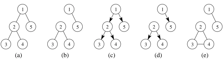
Figure 1: Graphical models on five nodes: (a) undirected spanning tree, (b) undirected non-spanning tree, (c) directed non-spanning tree, (d) directed non-non-spanning tree, (e) undirected clusters.
that is, the tree may consist of multiple connected components (such a graph is sometimes referred to as a “forest”). A spanning tree is a tree that includes all of the nodes in the graph (see Figure 1 for examples).
A probability distribution on an undirected graphical model is generally defined as a product of functions defined on the cliques of the graph. The cliques in an undirected tree are pairs of nodes and single nodes; thus, to parameterize a probability distribution on a tree, we define func-tions ψuv(xu,xv) andψu(xu), for (u,v)∈
E
, and u∈V
, respectively. These potential functionsare nonnegative, but otherwise arbitrary. The joint probability is defined as a product of potential functions:
p(x) = 1
Z(u
∏
,v)∈Eψuv(xu,xv)∏
v∈Vψu(xu), (1)
where Z is a normalization factor. Ranging over all possible choices of potential functions, we obtain a family of probability distributions associated with the given tree. We say that the members of this family factorize according to T .
Given a graphical model, we want to be able to compute marginal and conditional probabilities of interest—the probabilistic inference problem. An algorithm known as the junction tree algorithm provides a general framework for solving the probabilistic inference problem for arbitrary graphs, but scales exponentially in the size of the maximal clique. In the case of trees, the junction tree algorithm reduces to a simpler algorithm known as the sum-product algorithm or belief propagation
algorithm. This algorithm yields marginal probabilities p(xu) and p(xu,xv), for all(u,v)∈
E
and for all u∈V
, in time proportional to the number of edges in the tree (Pearl, 2000). The existence of this algorithm is one of the major justifications for restricting ourselves to trees.The functions ψuv(xu,xv) and ψu(xu) are arbitrary nonnegative functions, and need have no
direct relationship to the marginal probabilities p(xu,xv)and p(xu). It turns out, however, that it is
in the following form:2
p(x) =
∏
(u,v)∈E
p(xu,xv) p(xu)p(xv)u∈
∏
Vp(xu). (2)
Note that this is a special case of Equation (1) in which the normalization factor is equal to one.
2.2 Directed Trees
A directed tree is a directed graph in which every node has at most one parent. We can obtain a directed tree from an undirected tree by choosing a founder node in each connected component and orienting all edges in that component to point away from the founder (in Figure 1, the founders were chosen to be the nodes numbered 1 and 2).
Probability distributions on directed graphs are defined in general in terms of products of con-ditional and marginal probabilities, one for each node. In the case of directed tree, letting
F
denote the set of founders, and lettingU
=V
\F
denote the remaining nodes, we obtain the following definition of the joint probability:p(x) =
∏
f∈F
p(xf)
∏
u∈Up(xu|xπu), (3)
whereπudenotes the parent of node u.
Note that Equation (3) is a special case of Equation (1), with normalizing constant Z equal to one. This supports our earlier contention that there are no differences in representational power between undirected and directed trees.
As we will see in Section 7, however, the fact that the normalizing constant Z is equal to one in the directed case is convenient for estimating the densities associated with a tree (once the matrix
W and the tree T have been determined). A log likelihood based on Equation (3) decouples into a
sum of logarithms of individual marginal and conditional probabilities, allowing us to decompose the density estimation problem into separate estimation problems.
2.3 Conditional Independence
Apart from being parsimonious probabilistic models, directed and undirected graphical models have an equivalent characterization based on conditional independence and graph separation. In the case of trees, this is particularly simple: under mild assumptions on the joint probability density of the random variables, the variables(x1, . . . ,xm)factorize according to the tree T if and only if, for any three subsets A, B, C of
V
, such that C separates A from B in the graph, then the set of variablesxA ={xi,i∈A}, xB ={xi,i∈B} and xC ={xi,i∈B} are such that xA is independent from xB
given xC (in the model (a) in Figure 1, we have for example{x3,x4} independent from x5 given x2). In particular, if there are two separate connected components, variables in different connected
components are independent from one another.
2.4 Non-Spanning Trees and Clusters
An exact (undirected) graphical model for clusters of variables would have no edges between nodes that belong to different clusters and would be fully-connected within a cluster (as illustrated in
Figure 1 for the clusters{1,5} and{2,3,4}). Using a non-spanning tree models inter-cluster in-dependence, while providing a rich but tractable model for intra-cluster in-dependence, by allowing an arbitrary pattern of tree-structured dependence within a cluster. In particular, learning the best possible non-spanning tree that fits a given distribution provides a way to learn the number and size of the clusters for that particular distribution.
3. Semiparametric Maximum Likelihood
In this section we derive the objective function that will be minimized to determine the demixing matrix W and the tree T in the TCA model with iid samples. Let x= (x1, . . . ,xm)> be an
m-component random vector with joint “target” distribution p(x). Our primary goal is to minimize the Kullback-Leibler (KL) divergence D(p||q) =Ep(x)logpq((xx)) between p(x) and our model q(x) of this vector. Typically, p(x)will be the empirical distribution associated with a training set and minimizing the KL divergence is well known to be equivalent to maximizing the likelihood of the data. In a semiparametric model, the parameters of interest—the matrix W and the tree T in our case—do not completely specify the distribution q(x); the additional (infinite-dimensional) set of parameters that would be needed to complete the specification are left unspecified. More precisely, we define our objective function for T and W to be a “profile likelihood”—the minimum of the KL divergence D(p||q)with respect to arbitrary distributions of the source components si(Murphy and
van der Vaart, 2000). As we will show, it turns out that this criterion can be expressed in term of mutual information terms relating components that are neighbors in the tree T . We first review the classical ICA setting where the components siare assumed independent. Then, we describe the case
where W is fixed to identity and T can vary—this is simply the tree model presented by Chow and Liu (1968). We finally show how the two models can be combined and generalized to the full TCA model where both W and T can vary.
In the following sections we generally label the nodes with integers; thus, we let
V
={1,2, . . . ,m}. We will work with the pairwise mutual information I(xu,xv) between two variables xu and xv,de-fined as I(xu,xv) =D(p(xu,xv)||p(xu)p(xv))and the m-fold mutual information I(x1, . . . ,xm), de-fined as I(x1, . . . ,xm) =D(p(x)||p(x1)· · ·p(xm)). Finally, all mutual informations, entropies and expectations are relative to the distributions p(x)or p(s)unless otherwise noted.
3.1 ICA Model
The classical ICA model takes the form x=As where A is an invertible mixing matrix and s has
independent components. If the variable x is Gaussian, then ICA is not identifiable, that is, the optimal matrix W =A−1 is only defined up to an orthogonal matrix. Thus, non-Gaussianity of components is a crucial assumption for a full ICA solution to be well-defined, and we also make this assumption throughout the current paper.3 However, the Gaussian case is still of interest because it allows us to reduce the size of the search space for W (see Section 4.2 and Appendix A for details). In addition, the Gaussian contrast function is a basis for the kernel generalized variance empirical contrast function presented in Section 5.3 and the Gaussian stationary time series contrast function in Section 8.
Given a random vector x with distribution p(x) (not necessarily having independent compo-nents), the distribution q(x)with independent components that is closest to p(x)in KL divergence is the product q(x) =p(x1)· · ·p(xm), and the minimum KL divergence is thus D(p(x)||p(x1)· · ·p(xn)),
which is exactly the mutual information I(x1, . . . ,xm).
We now turn to the situation where A can vary. Letting W =A−1, we let
D
W denote the set of all distributions q(x) such that s=W x has independent components. Since the KL divergence isinvariant under an invertible transformation, the best approximation to p(x)by a distribution in
D
W is obtained as the product of the marginals of s=W x, which yields:min
q∈DWD(p||q) =I(s1, . . . ,sm). (4)
Thus, in the semiparametric ICA approach, we wish to minimize the mutual information of the estimated components s=W x. We will generalize Equation (4) to the TCA model in Section 3.4.
In practice, we do not know the density p(x)and thus the estimation criteria must be replaced by functionals of the sample data, functionals that are referred to as “empirical contrast functions.” Classical ICA contrast functions involve either approximations to the mutual information or alter-native measures of dependence involving higher-order moments (Cardoso, 1999, Hyv ¨arinen et al., 2001b, Pham, 2001b).
3.2 Chow-Liu Algorithm and T -Mutual Information
Given an undirected tree T on the vertices
V
={1, . . . ,m}, we letD
T denote the set of probability distributions q(x) that factorize according to T . We want to model p(x) using a distribution q(x)in
D
T. Trees are a special case of decomposable models and thus, for a given tree T , minimizing the KL divergence is straightforward and yields the following “Pythagorean” expansion of the KL divergence (Jirousek, 1991):Theorem 1 For a given tree T(
V
,E
)and a target distribution p(x), we have, for all distributions q∈D
T,D(p||q) =D(p||pT) +D(pT||q), (5)
where pT(x) =∏(u,v)∈E p(xu,xv)
p(xu)p(xv)∏u∈V p(xu). In addition, q=pT minimizes D(p||q)over q∈
D
T,
and we have:
IT(x) = min
q∈DTD(p||q) =D(p||pT) = I(x1, . . . ,xm)−
∑
(u,v)∈E
I(xu,xv). (6)
Proof Let q be a distribution in
D
T, that is such that q(x) =∏(u,v)∈Eqq(x(uxu)q,x(vx)v)∏u∈Vq(xu). Since the density of q(x)is a product of functions of pairs of variables linked by an edge and of functions of single variables, and since p(x)and pT(x)have the same marginal distributions on the cliques ofwe get Ep(x)log pT(x) =EpT(x)log pT(x). We thus have:
D(p(x)||q(x)) = Ep(x)log p(x)−Ep(x)log q(x) = Ep(x)log p(x)−EpT(x)log q(x)
= Ep(x)log p(x)−EpT(x)log pT(x) +EpT(x)log pT(x)−EpT(x)log q(x) = Ep(x)log p(x)−Ep(x)log pT(x) +EpT(x)log pT(x)−EpT(x)log q(x) = D(p(x)||pT(x)) +D(pT(x)||q(x)),
which proves the Pythagorean identity; this in turn implies that the distribution in
D
T with mini-mum KL divergence is indeed pT. We can now compute D(p||pT)as follows (entropy and mutualinformation terms are computed using the distribution p(x)):
D(p(x)||pT(x)) = Ep(x)log p(x)−Ep(x)log pT(x)
= −H(x)−
∑
(u,v)∈E
Ep(x)log
p(xu,xv) p(xu)p(xv)
−
∑
u∈VEp(x)log p(xu)
= −H(x)−
∑
(u,v)∈E
I(xu,xv) +
∑
u∈VH(xu)
= I(x1, . . . ,xm)−
∑
(u,v)∈E
I(xu,xv)
We refer to IT(x)in Equation (6) as the T -mutual information: it is the minimum possible loss of information when encoding the distribution p(x) with a distribution that factorizes in T . It is equal to zero if and only if p does factorize according to T . Such a quantity can be defined for any directed or undirected graphical model and can be computed in closed form for all directed graphical models and all decomposable undirected graphical models (Dawid and Lauritzen, 1993, Friedman and Goldszmidt, 1998).
In order to find the best tree T , we need to minimize IT(x)in Equation (6) with respect to T . Without any restriction on T , since all mutual information terms are nonnegative, the minimum is attained at a spanning tree and thus the minimization is equivalent to a maximum weight spanning tree problem with (nonnegative) weights I(xu,xv), which can be solved in polynomial time by greedy algorithms (see next section and Cormen et al., 1989).
3.3 Prior Distributions on Trees
In order to allow non-spanning trees in our model, we include a prior term w(T) =log p(T)where
p(T)is a prior probability on the forest T which penalizes dense forests. In order to be able to find a global minimum of IT(x)−w(T)using greedy algorithms, we restrict the penalty w(T)to be of the
form w(T) =∑(u,v)∈Ew0uv+f(#(T)), where w0uv is a fixed set of weights, f is a concave function,
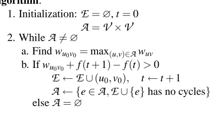
and #(T) is the number of edges in T . We use the algorithm outlined in Figure 2, with weights
wuv=I(xu,xv) +w0uv: starting from the empty graph, while it is possible, incrementally pick a safe
Input: weights{wuv,u,v∈
V
}, concave function f(t)Algorithm:
1. Initialization:
E
=∅, t=0A
=V
×V
2. While
A
6=∅a. Find wu0v0 =max(u,v)∈Awuv
b. If wu0v0+f(t+1)−f(t)>0
E
←E
∪(u0,v0), t←t+1A
← {e∈A
,E
∪ {e}has no cycles}else
A
=∅Output: maximum weight forest T(
V
,E)Figure 2: Greedy algorithm for the maximum weight forest problem.
Proposition 2 If J(T)has the form J(T) =∑(u,v)∈Ewuv+f(#(T))where{wuv,u,v∈
V
}is a fixed set of weights, and f is a concave function, then the greedy algorithm outlined in Figure 2 outputsthe global maximum of J(T)over all forests.
The magnitude of the weights w(T) provides a way to control the degree of sparsity of the resulting tree: if the weights w0uvare negative and have large magnitude, then additional edges are heavily penalized and the tree will tend to have a small number of edges. We can set the weights by casting the problem of finding the best forest as a model selection problem for graphical models and use classical model selection criteria, such as the Akaike information criterion (AIC) or the Bayesian information criterion (BIC) (Heckerman et al., 1995, Hastie et al., 2001, Bach and Jordan, 2003). In simulations, we used a constant negative penalty for each edge.
3.4 TCA Model
In TCA, we wish to model the variable x using the model x=As, where A is an invertible mixing
matrix and s factorizes in a tree T . Letting W =A−1, we let
D
W,T denote the set of all such distribu-tions. The KL divergence is invariant by invertible transformation of its arguments, so Theorem 1 can be easily extended:Theorem 3 If x has distribution p(x), then the minimum KL divergence between p(x)and a distri-bution q(x)∈
D
W,T is equal to the T -mutual information of s=W x, that is:J(x,W,T) = min
q∈DW,TD(p||q) =I
T(s) (7)
= I(s1, . . . ,sm)−
∑
(u,v)∈E
I(su,sv). (8)
Therefore, in the semiparametric TCA approach, we wish to minimize J(x,W,T)with respect to W and T .
information: indeed the interplay between the 2-fold and m-fold mutual information terms is crucial, making it possible to avoid overcounting or undercounting the pairwise dependencies. The contrast functions that we propose thus have such a link—our first two contrast function approximates the mutual information terms directly, and our third proposed contrast function has an indirect link to mutual information. Before describing these three contrast functions, we turn to the description of the main properties of the TCA model.
4. Properties of the TCA Model
In this section we describe some properties of the TCA model, relating them to properties of the simpler ICA model. In particular we focus on identifiability issues and on the Gaussian case.
4.1 Identifiability Issues
In the ICA model, it is well known that the matrix W can only be determined up to permutation or scaling of its rows. In the TCA model, we have the following set of indeterminacies. Note that this set of indeterminacies is only necessary and may not be sufficient in general.
• Permutation of components. W can be premultiplied by a permutation matrix without changing the value of J(x,W,T), as long as the tree T is also permuted analogously. This implies that in principle we don’t have to consider all possible trees, but just equivalence classes under vertex permutation. Our empirical contrast functions are invariant with respect to that invariance. Therefore, it can be safely, although slightly inefficiently, ignored.
• Scaling of the components. W can be premultiplied by any invertible diagonal matrix. Thus we can restrict our search to components that have unit variance.
• Rotation of connected components of size two. If the tree T is non-spanning and has more than one connected component, then for each component C of size two, W can be premulti-plied by any linear transform that leaves all other components invariant and the component C globally invariant. When identifying clusters instead of forests, then, as shown by Cardoso (1998), the demixing matrix is identifiable only up to the p subspaces spanned by the set of rows corresponding to each of the p components. However, this does not hold in general in the tree-structured case which imposes further constraints for connected components of size larger than three. This invariance is a special case of the leaf mixing invariance that we now present.
• Mixing of a leaf node with its parent. For a given tree structure T , and a leaf node c, adding a multiple of the value of its parent p to the value of the leaf will not change the goodness of fit of the tree T (see Figure 3). Indeed, a leaf node is only present in the likelihood through the conditional probability p(sc|sp), and thus we can equivalently model p(sc|sp)
or p(λsc+µsp|sp) for any µ and any non-zero λ. The T -mutual information IT(s) is thus invariant under such transformations.
s
s
pc
Figure 3: Leaf mixing invariance. See text for details.
example by requiring marginal decorrelation. However, this normalization depends on the tree, so it is not appropriate when comparing trees. Instead, we simply add a penalty term to our contrast functions, penalizing the correlation between components that are linked by an edge of the tree T (see Section 6 for details).
4.2 The Gaussian Case
In the ICA model, if the variable x is Gaussian, the solutions are the matrices W that make the covariance matrix of s=W x equal to identity. Thus, they are defined up to an orthogonal matrix R.
In the TCA model, with a fixed tree T , there is more than one covariance matrix that leads to a tree-structured graphical model with graph T for the underlying Gaussian random vector. For a Gaussian random vector, conditional independences can be read out from zeros in the inverse of the covariance matrix (e.g. Lauritzen, 1996). Applying this result to trees, we get
Proposition 4 If x= (x1, . . . ,xm) is Gaussian with covariance matrix Σ, it factorizes in the tree T(
V
,E
)if and only if for all(u,v)∈/E
, we have(Σ−1)uv=0.Let
C
T denote the set of all covariance matrices that respect these constraints. Note that it is pos-sible to give a constructive description of this set, simply by writing down the factorization in any directed tree associated with the undirected tree T , using linear Gaussian conditional probability distributions (Luettgen et al., 1994). The number of degrees of freedom in such a construction is 2m−1 if no constraint is imposed on the variance of the components, and m−1 if the components are constrained to have unit variance.Finally, we can compute IT(Σ) =IT(x)for a Gaussian variable x with covariance matrixΣ:
IT(Σ) =IG(Σ)−
∑
(u,v)∈E
IuvG(Σ), (9)
where IG(Σ) =−12logΣ11···detΣΣ
mm is the m-fold mutual information between x1, . . . ,xm and I
G uv(Σ) = −1
2log
ΣuuΣvv−Σ2uv
ΣuuΣvv is the pairwise mutual information between xuand xv. We then have the appealing property that for any positive definite matrixΣ,Σ∈
C
T if and only if IT(Σ) =0. Once the setC
Tis well defined, we can easily solve TCA in the Gaussian case, as the following theorem makes precise:
Theorem 5 If x1, . . . ,xmare jointly Gaussian with covariance matrixΣ, the variable s=W x
fac-torizes in the tree T if and only if there exists an orthogonal matrix R and C∈
C
T such thatW=C1/2RΣ−1/2.
Second, the Gaussian solution can be exploited to yield a principled reduction of the search space for W . Recall that in ICA it is common to “whiten” (i.e. decorrelate and normalize) the data in a pre-processing step; once this is done the matrix W can be constrained to be an orthogonal matrix. In the TCA model, we cannot always require decorrelation of the components; indeed, two components linked by an edge might be heavily correlated. However, in some specific situations (Hyv ¨arinen et al., 2001a), or when looking for clusters, it is appropriate to look for uncorrelated components and whitening can then be used to limit the search space for the matrix W .
If it is not possible to whiten the data, it seems reasonable for a given tree T to constrain W to be such that it is a solution to the Gaussian relaxation of the problem. This cannot be achieved entirely, because if a distribution factorizes in T , a Gaussian variable with the same first and second order moments does not necessarily factorize according to T (marginal independencies are preserved, but conditional independencies are not); nevertheless, such a reduction in complexity in the early stages of the search is very helpful to the scalability of our methods to large m, as discussed in Appendix A. We now turn to the definitions of our three empirical contrast functions for TCA.
5. Estimation of the Contrast Function
We have developed three empirical contrast functions. Each of them is derived from a corresponding ICA contrast function, extended to the TCA model.4
5.1 Estimating Entropies Using Kernel Density Estimation
Our first approach to approximating the objective function J(x,W,T)is a direct approach, based on approximating the component marginal entropies H(su)and joint entropies H(su,sv), H(s)and H(x)
via kernel density estimation (KDE; Silverman, 1985, Pham, 1995). The first term in J(x,W,T)
can be written as I(s1, . . . ,sm) =∑uH(su)−H(s), which can be expanded into∑uH(su)−H(x)−
log|detW|. Since the joint entropy H(x) is constant we do not need to compute it and thus to estimate I(s1, . . . ,sm) we need only estimate one-dimensional entropies H(si). We also require
estimates of the pairwise mutual information terms in the definition of J(x,W,T), which we obtain using two-dimensional entropy estimates. Thus, letting ˆHuand ˆHuvdenote estimates of the singleton and pairwise entropies, respectively, we define the following empirical contrast function:
JKDE=
∑
u
ˆ
Hu−
∑
(u,v)∈E
(Hˆu+Hˆv−Hˆuv)−log|detW|. (10)
Given a set of N training samples {xi} inRd and a kernel in Rd, that is, a nonnegative function K :Rd→Rthat integrates to one, the kernel density estimate with bandwidth h is defined as ˆf(x) =
1 Nhd ∑
N
i=1K x−xhi
(Silverman, 1985). In this paper we use Gaussian kernels K(x) = (2π1)d/2e−||x|| 2/2
with d=1,2.
The entropy of x is estimated by evaluating ˆf(x) at points on a regular mesh that spans the support of the data, and then performing numerical integration. Binning, together with the fast Fourier transform, can be used to speed up the evaluations, resulting in a complexity which is linear in N and depends on the number M of grid points that are required. Although automatic methods
exist for selecting the bandwidth h (Silverman, 1985), in our experiments we used a constant h=
0.25. We also fixed M=64.
Although each density estimate can be obtained reasonably cheaply, we have to perform O(m2)
of these when minimizing over the tree T . This can become expensive for large m, although, as we show in Appendix A, this cost can be reduced by performing optimization on subtrees. In any case, our next two contrast function are aimed at handling problems with large m.
5.2 Gram-Charlier Expansions
A contrast function based on cumulants is easily derived from Equation (10), using Gram-Charlier expansions to estimate one-dimensional and two-dimensional entropies, as discussed by Amari et al. (1996) and Akaho et al. (1999). Since this contrast function only involves up to fourth order cu-mulants, it is numerically efficient and can be used to rapidly find an approximate solution which can serve as an initialization for the slower but more accurate contrast functions based on the other estimation methods (KGV or KDE).
More precisely, to compute the entropy of a centered univariate random variable a, we define
r=a/σwhereσ2=var(a). We have the following approximation:
H(a) =H(r) +logσ≈1
2log(2πeσ
2)− 1
48(Er
4−3)2− 1
12(Er
3)2.
In order to compute the joint entropy of two centered univariate variables a and b, we let r and s denote the corresponding “whitened” variables, i.e. such that(r,s)>=C−1/2(a,b)>, where C is the 2×2 covariance matrix of a and b. The entropy H(a,b)can be computed from the entropy H(r,s)
as H(a,b) =H(r,s) +1
2log detC; for H(r,s), we have the following approximation (Akaho et al.,
1999):
H(r,s)≈log 2πe− 1
12
(Er3)2+ (Es3)2+3(Er2s)2+3(Ers2)2 − 1
48
(Es4−3)2+ (Er4−3)2+6(Er2s2−1)2+4(Er3s)2+4(Ers3)2
.
Thus we can compute estimates ˆHuv and ˆHu as in previous section and define a contrast function
JCU M.
5.3 Kernel Generalized Variance
Our third contrast function is based on the kernel generalized variance, an approximation to mutual information introduced by Bach and Jordan (2002). We begin by reviewing the kernel general-ized variance, emphasizing a simple intuitive interpretation. For precise definitions and properties, see Bach and Jordan (2002).
5.3.1 APPROXIMATION OFMUTUALINFORMATION
Let x= (x1, . . . ,xm)>be a random vector with covariance matrixΣ. The m-fold mutual information
for an associated Gaussian random vector with same mean and covariance matrix as x is equal to
IG(Σ) =−12log
detΣ
Σ11···Σmm
. The ratio Σ11···detΣΣ
and then treat the mapped variables as Gaussian in this space, it turns out that we obtain a useful approximation of the mutual information. More precisely, we map each component xitoΦ(xi)∈
F
via a mapΦ, and define the covariance matrix
K
ofΦ(x) = (Φ(x1), . . . ,Φ(xm))T ∈F
mby blocks:K
i jis the covariance betweenΦ(xi)andΦ(xj). The size of each of these blocks is the dimension ofF
. For simplicity we can think ofF
as a finite-dimensional space, but the definition can be general-ized to any infinite-dimensional Hilbert space. LetΦG(x)∈F
mbe a Gaussian random vector withthe same mean and covariance asΦ(x). The mutual information IK(
K
)betweenΦG1(x), . . . ,ΦGm(x)
is equal to
IK(
K
) =−12log
detK det
K
11· · ·detK
mm, (11)
where the ratio detK11···detdetK K
mm is called the kernel generalized variance (KGV).
We now list the main properties of IK, which we refer to as the KGV-mutual information.
• Mercer kernels and Gram matrices. A Mercer kernel onRis a function k(x,y)fromR2toR
such that for any set of points{x1, . . . ,xN}inR, the N×N matrix K, defined by Ki j=k(xi,xj),
is positive semidefinite. The matrix K is usually referred to as the Gram matrix of the points
{xi}. Given a Mercer kernel k(x,y), it possible to find a space
F
and a mapΦ fromR toF
, such that k(x,y)is the dot product inF
betweenΦ(x)andΦ(y)(see, e.g., Sch ¨olkopf and Smola, 2001). The spaceF
is usually referred to as the feature space and the mapΦas thefeature map. This allows us, given sample data, to define an estimator of the KGV via the
Gram matrices Kiof each component xi. Indeed, using the “kernel trick,” we can find a basis
of
F
whereK
i j =KiKj. Thus, for the remainder of the paper, we assume thatΦandF
areassociated with a Mercer kernel k(x,y).
• Linear time computation. If k(x,y) is the Gaussian kernel k(x,y) =exp(−(x−y)2/2σ2),
then the estimator based on Gram matrices can be computed in linear time in the number
N of samples. In this situation,
F
is an infinite-dimensional space of smooth functions.This low complexity is obtained through low-rank approximation of the Gram matrices using incomplete Cholesky decomposition (Bach and Jordan, 2002). We need to perform m such decompositions, where each decomposition is O(N). The worst-case running time complexity is O(mN+m3), but under a wide range of situations, the Cholesky decompositions are the practical bottlenecks of the evaluation of IK, so that the empirical complexity is O(mN).
• Relation to actual mutual information. For m=2, when the kernel widthσtends to zero, the KGV mutual information tends to a quantity that is an expansion of the actual mutual information around independence (Bach and Jordan, 2002). In addition, for any m, IK is a valid contrast function for ICA, in the sense that it is equal to zero if and only if the variables
x1, . . . ,xmare pairwise independent.
• Regularization. For numerical and statistical reasons, the KGV has to be regularized, which amounts to convolving the Gaussian variableΦG(x)by another Gaussian having a covariance matrix proportional to the identity matrixκI. This implies that in the approximation of the
KGV, we have
K
i j =KiKj for i6= j, andK
i j = (Ki+NκI)2for i= j, whereκis a constant5.3.2 A KGV CONTRASTFUNCTION FORTCA
Mimicking the definition of the T -mutual information in Equation (6) and the Gaussian version in Equation (9), we define the KGV contrast function JK(x,T) for TCA as JK(x,T) =IK(x)−
∑(u,v)∈EIuvK(x), that is:
JK(x,T) =−1
2log
det
K
detK
11· · ·detK
mm+1
2(u,
∑
v)∈Elogdet
K
uv,uvdet
K
uudetK
vv.
An important feature of JK is that it is the T -mutual information ofΦG1(x), . . . ,ΦG
m(x), which are
linked to x1, . . . ,xmby the feature maps and the “Gaussianization.” It is thus always nonnegative.
Note that going from a random vector y to its associated Gaussian yGis a mapping from distribution to distribution, and not a mapping from each realization of y to a realization of yG. Unfortunately, this mapping preserves marginal independencies but not conditional independencies, as pointed out in Section 4.2. Consequently, JK(x,T)does not characterize factorization according to T ; that is,
JK(x,T)might be strictly positive even when x does factorize according to T . Nonetheless, based on our earlier experience with KGV in the case of ICA (Bach and Jordan, 2002), we expect JK(x,T)to provide a reasonable approximation to IT(x). Intuitively, we fit the best tree for the Gaussians in the feature space and hope that it will also be a good tree in the input space. Recent work by Fukumizu et al. (2003) has shown how to use KGV to exactly characterize conditional independence.
Numerically, JK(x,T) behaves particularly nicely, since all of the quantities needed are Gram matrices, and are obtained from the m incomplete Cholesky decompositions. Thus we avoid the
O(m2)complexity. In our empirical experiments, we used the settingsσ=1 andκ=0.01 for the free parameters in the KGV. The contrast function that we minimize with respect to T and W is then
JKGV(x,W,T) =JK(W x,T).
6. The TCA Algorithm
We now give a full description of the TCA algorithm. Any of the three contrast functions that we have defined can be used in the algorithm. We generically denote the contrast function as J(x,W,T)
in the following description of the algorithm.
6.1 Formulation of the Optimization Problem
First, as noted in Section 4.1, we minimize J(x,W,T) on the space of matrices such that W x has unit variance components. That is, ifΣdenotes the covariance matrix of x, we constrain the rows of
WΣ1/2 to have unit norm. Therefore, the search space
M
is isomorphic to a product of m spheres in m dimensions. In order to take into account the “leaf mixing” invariance (see Section 4.1), we also add a penalty term, JC(x,W,T) =−12∑(u,v)∈Elog 1−corr2((W x)u,(W x)v)
that penalizes marginal correlation along edges of the tree T . Finally, a prior term w(T)may be added, as defined in Section 3.3.
We thus aim to solve the following optimization problem over W and T :
minimize F(W,T) =J(x,W,T) +λCJC(x,W,T)−w(T)
subject to (WΣW>)ii=1,∀i∈ {1, . . . ,m},
whereλC determines how much we penalize the marginal correlations. In all of our experiments
formulation simplifies as follows, with a search space
M
isomorphic to the group of orthogonal matrices:minimize Fw(W,T) =J(x,W,T)−w(T)
subject to WΣW>=I,
6.2 Minimization Algorithm
The optimization problem that we need to solve involves one continuous variable W and one discrete variable T . Minimization with respect to any of the two variables while the other is fixed can be done efficiently: minimizing with respect to T is equivalent to a maximum weight forest problem, which can easily be solved by the greedy algorithm presented in Section 3.3, while minimizing with respect to W can be done by gradient descent—for the three empirical contrast functions defined in Section 5, there are efficient techniques to compute the gradient (Silverman, 1985, Akaho et al., 1999, Bach and Jordan, 2002). However, since one of the two variables is discrete, an alternating minimization procedure might not exhibit good convergence properties. In order to use continuous optimization techniques, we consider the function G(W) obtained by minimizing with respect to the tree T ; that is, G(W) =minTF(W,T). This function is continuous and piecewise differentiable.
The problem is now that of minimizing this function with respect to W on a manifold
M
, which in our situation, is a product of spheres in the general case or the orthogonal group when the whitening constraint is imposed. We can use the structure of such manifolds to design efficient coordinate descent algorithms; indeed it is possible to minimize functions defined on those manifolds with an iterative procedure: at each iteration, a pair of indices (i,j) is chosen, then all the rows of W are held fixed except the i-th and j-th row which are allowed to vary inside the subspace spanned by the i-th and j-th rows obtained from the previous iteration. For both types of manifold, all elements can be generated by a finite sequence of such local moves.In the case of the orthogonal group, this is the classical technique of Jacobi rotations (Cardoso, 1999) where for each pair (i,j)we have to solve a one-dimensional problem. In the case of the product of spheres, this is a two-dimensional problem. For both problems, the evaluation of the contrast functions when all rows but two are held fixed has linear complexity in m, thus making the local searches efficient. An outline of the algorithm is presented in Figure 4. At the obtained stationary point W , if there is only one tree that attains the minimum minTF(W,T), then this is
a local minimum of G(W). We present in Appendix A a set of techniques to make the algorithm scalable to large numbers of variables.
7. TCA as a Density Estimation Model
TCA can be used as a density estimation model. Indeed, once the optimal (or an approximation thereof) W and T are found, we just need to perform density estimation in a graphical model, independently of the method that was used to find W and T . The model with respect to which we carry out this density estimation is a tree, and thus we can work either within the directed graphical model framework or the undirected graphical model framework. We prefer the former because the lack of a normalizing constant implies that the density estimation problem decouples.
We thus have to estimate a density of the form p(s) =∏f∈F p(sf)∏u∈V\F p(su|sπu), where
F
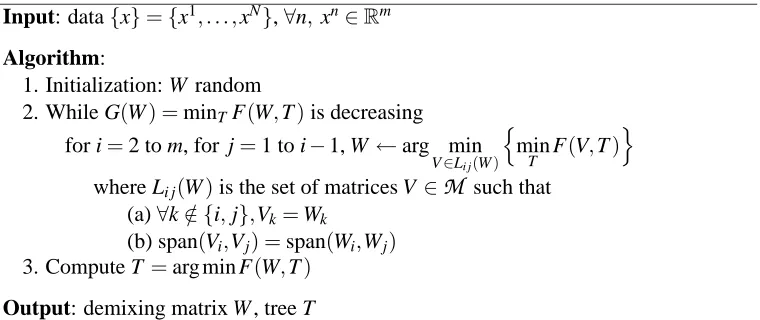
is a set of founders for the directed tree T andπuis the parent of node u in the directed tree T . TheInput: data{x}={x1, . . . ,xN},∀n,xn∈Rm
Algorithm:
1. Initialization: W random
2. While G(W) =minTF(W,T)is decreasing
for i=2 to m, for j=1 to i−1, W ←arg min
V∈Li j(W)
n
min
T F(V,T)
o
where Li j(W)is the set of matrices V∈
M
such that(a)∀k∈ {/ i,j},Vk=Wk
(b) span(Vi,Vj) =span(Wi,Wj)
3. Compute T =arg min F(W,T)
Output: demixing matrix W , tree T
Figure 4: The TCA algorithm: F(W,T)is the contrast function and
M
is the search space for W , as defined in Section 6.1 (we use the notation Akfor the k-th row of a matrix A).for nodes with no parents (the founders), and conditional density estimates for the remaining nodes with one parent. In this paper we use a Gaussian mixture model for the densities at the founders, and conditional Gaussian mixture models, also known as “mixtures of experts models” (Jacobs et al., 1991), for the remaining conditional probabilities. All of these mixture models can be estimated via the expectation-maximization (EM) algorithm. In order to determine the number of mixing components for each model, we use the minimum description length criterion (Rissanen, 1978).
Our two-stage approach is to be contrasted with an alternative one-stage approach in which one would define a model using W , T and Gaussian-mixture conditional distributions, and perform max-imum likelihood using EM—such an approach could be viewed as an extension of the independent factor analysis model (Attias, 1999) to the tree setting. By separating density estimation from the search for W and T , however, we are able to exploit the reduction of our parameter estimation prob-lem to bivariate density estimation. Bivariate density estimation is a well-studied probprob-lem, and it is possible to exploit any of a number of parametric or nonparametric techniques. These techniques are computationally efficient, and good methods are available for controlling smoothness. We also are able to exploit the KGV technique within the two-phase approach, an alternative that does not rely explicitly on density estimation.
Finally, and perhaps most significantly, our approach does not lead to intractable inference prob-lems that require sampling or variational methods, as would be necessary within a tree-based gen-eralization of the independent factor analysis approach.5
8. Stationary Gaussian Processes
Pham (2002) has shown that for ICA, the semiparametric approach can be extended to stationary Gaussian processes. In this section, we extend his results to the TCA model. We assume first that the sources are doubly-infinite sequences of real valued observations {sk(t),t∈Z}, k=1, . . . ,m.
We model this multivariate sequence as a zero-mean multivariate Gaussian stationary process (we assume that the mean is zero or has been removed). We letΓ(h), h∈Z, denote the m×m matrix
autocovariance function, defined as:
Γ(h) =E[s(t)s(t+h)>].
We assume that∑∞−∞||Γ(h)||<∞, so that the spectral density matrix f(ω)is well-defined:
f(ω) = 1
2π +∞
∑
h=−∞Γ(h)e−ihω.
For each ω, f(ω) is an m×m Hermitian positive semidefinite matrix. In addition the function
ω7→ f(ω)is 2π-periodic. In the following we always assume that for everyω, f(ω) is invertible (i.e., positive definite).
8.1 Entropy Rate of Gaussian Processes
The entropy rate of a process s is defined as (Cover and Thomas, 1991)
H(s) = lim
T→∞
1
TH(s(t), . . . ,s(t+T)).
In the case of Gaussian stationary processes, the entropy rate can be computed using the spectral density matrix (due to an extension of Szeg ¨o’s theorem to multivariate processes, see e.g. Hannan, 1970):
H(s) = 1
4π
Z π −πlog det
[4π2e f(ω)]dω.
Note that this is an analog of the expression for the entropy of a Gaussian vector z with covariance matrixΣ, where H(z) = 12log det[2πeΣ].
By the usual linear combination of entropy rates, the mutual information between processes can be defined. Also, we can express the entropy rate of the process x=V s, where V is a d×m matrix,
using the spectral density of s:
H(V s) = 1
4π
Z π
−πlog det[4π
2eV f(ω)V>]dω.
8.2 Graphical Model for Time Series
The graphical model framework can be extended to multivariate time series (Brillinger, 1996, Dahlhaus, 2000). The dependencies that are considered are between whole time series; that is, between the entire sets{si(t),t∈Z}, for i=1, . . .m. If the process is jointly Gaussian and
station-ary, then most of the graphical model results for Gaussian variables can be extended. In particular, sa
is conditionally independent from sbgiven all others su,u6=a,b, if and only if∀ω,(f(ω)−1)ab=0.
8.3 Contrast Function
Let x be a multivariate time series{xk(t),t∈Z}, k=1, . . . ,m. We wish to model the variable x using
the model x=As, where A is an invertible mixing matrix and s is a Gaussian stationary time series
that factorizes in a forest T . Letting W=A−1, we let
D
Wstat,T denote the set of all such distributions. We state without proof the direct extension of Theorem 3 to time series (Wudenotes the u-th row of W ):Theorem 6 If x has a distribution with spectral density matrix f(ω), then the minimum KL diver-gence between p(x)and a distribution q(x)∈
D
statW,T is equal to the T -mutual information of s=W x, that is:JSTAT(f,T,W) =IT(f,W) =I(f,W)−
∑
(u,v)∈E
Iuv(f,W), (12)
where
I(f,W) =− 1
4π
Z π −πlog
detW f(ω)W> W1f(ω)W1>· · ·Wmf(ω)Wm>
dω
is the m-fold mutual information between s1, . . . ,smand
Iuv(f,W) =−
1 4π Z π −π log (
1− Wuf(ω)W > v
2
Wuf(ω)Wu>·Wvf(ω)Wv>
)
dω
is the pairwise mutual information between suand sv.
Thus, the goal of TCA is to minimize JSTAT(f,T,W) =IT(f,W)in Equation (12) with respect to W and T ; in our simulations, we refer to this contrast function as the STAT contrast function.
8.4 Estimation of the Spectral Density Matrix
In the presence of a finite sample{x(t),t=0, . . . ,N−1}, we use the smoothed periodogram (Brock-well and Davis, 1991) in order to estimate the spectral density matrix at points ωj =2πj/N,
ωj∈[−π,π]. At those frequencies, the periodogram is defined as6
IN(ωj) =
1
N N
∑
t=1xte−itωj
!
N
∑
t=1xte−itωj
!>
,
and can readily be computed using m fast Fourier transforms (FFT). We use the following estimated spectral density matrices:
ˆ
f(ωk) =
1
N N−1
∑
j=0W(j)IN(ωj+k), (13)
where W(j)is a smoothing window that is required to be symmetric and sum to one. In our simula-tions, we used a Gaussian window W(j)∝e−j2/p2. If the number of samples N tends to infinity with
p(N)tending to infinity such that p(N)/N→0, then Equation (13) provides a consistent estimate of the spectral density matrix, and there are methods to select an optimal smoothing parameter p automatically (Ombao et al., 2001).
Finally, our contrast function involves integrals of the form
Z π
−πB(f(ω))dω.
Following Pham (2001a), we estimate them by Riemannian sums using estimated values of f at ωj=2πj/N,ωj∈[−π,π], from Equation (13). Because of the smoothness of the spectral density,
the Riemannian sums can be subsampled; in simulations we use 64 samples.
9. Simulation Results
We have conducted an extensive set of experiments using synthetic data.7 In a first set of experi-ments, we focus on the performance of the first stage of the algorithm, i.e., the optimization with respect to W and T , when the data actually follow the TCA model. In a second set of experiments, we focus on the density estimation performance, in situations where the TCA model assumptions actually hold, and in situations where they do not. Finally, in a third set of experiments, we focus on the task of recovering clusters in ICA, both in the non-Gaussian temporally independent case and the stationary Gaussian case.
9.1 Recovering the Tree and the Linear Transform
In this set of experiments, for various numbers of variables m, we generated data from distributions with known density: we selected a spanning tree T at random, and conditional distributions were selected among a given set of mixtures of experts. Then 1000 samples were generated and rotated using a known random square matrix A, which corresponds to a demixing matrix W =A−1.
To evaluate the results ˆW and ˆT of the TCA algorithm—with the three contrast function JCU M,
JKGV and JKDE, based on cumulants, the kernel generalized variance, and kernel density estimation, respectively—we need to use error measures that are invariant with respect to the known invariances of the model, as discussed in Section 4.1.
For the demixing matrix W , we use a measure commonly used for ICA (Amari et al., 1996), that is invariant by permutation and scaling of rows: we form B=WWˆ −1 and compute d =
100 m(m−1)∑
m i=1
n∑m j=1|Bi j|
maxj|Bi j|−1
o
. This measure is always between 0 and 100 and equal to zero if and
only if there is a perfect match between W and ˆW . Intuitively, it measures the average proportion of
components that are not recovered. However, because of the “leaf mixing” invariance, before com-puting d, we transform W and ˆW to equivalent demixing matrices which respect the normalization
we choose—marginal decorrelation between the leaf node and its parent. We let eW denote the final
error measure.
In order to compare the trees T and ˆT , we note that the computation of eW also outputs, for each estimated component, the true component that is closest. Using these assignments, we compute the number of edges in T that are not recovered in ˆT , and define the error eT as this number multiplied
by m−1100 (if two components are assigned to the same true component, which can only occur when the demixing is especially bad, then some edges of ˆT become trivial when estimated components
are assigned to true component, simply making eT larger).
We report results (averaged over 20 replications) in Table 1. We also ran two ICA algorithms, JADE (Cardoso, 1999) and Fast-ICA (Hyv¨arinen et al., 2001b). Our algorithms manage to recover
eW eT
ICA TCA TCA
m F-ICA JADE CUM KGV KDE CUM KGV KDE
4 34.1 20.9 7.3 2.9 1.8 0 0 0
6 33.2 21.6 9.3 3.9 2.0 8.5 1.5 1.5
8 30.5 17.4 10.8 6.2 2.3 14.5 8.2 2.9
12 25.2 16.4 10.7 6.6 2.3 31.8 9.5 5.5
16 24.1 15.8 12.0 7.0 1.5 34.1 12.4 2.5
Table 1: Recovering the tree T and the matrix W , for increasing numbers m of components. See text for details on the definitions of the performance measures eW and eT.
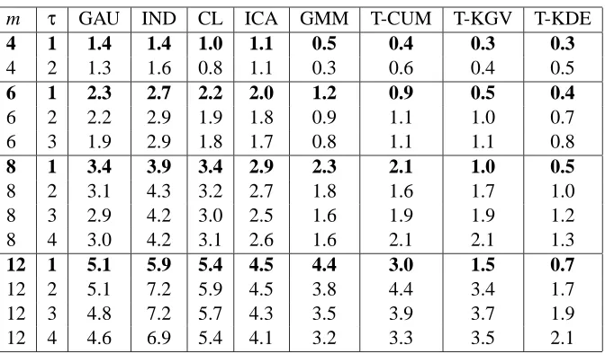
m τ GAU IND CL ICA GMM T-CUM T-KGV T-KDE
4 1 1.4 1.4 1.0 1.1 0.5 0.4 0.3 0.3
4 2 1.3 1.6 0.8 1.1 0.3 0.6 0.4 0.5
6 1 2.3 2.7 2.2 2.0 1.2 0.9 0.5 0.4
6 2 2.2 2.9 1.9 1.8 0.9 1.1 1.0 0.7
6 3 1.9 2.9 1.8 1.7 0.8 1.1 1.1 0.8
8 1 3.4 3.9 3.4 2.9 2.3 2.1 1.0 0.5
8 2 3.1 4.3 3.2 2.7 1.8 1.6 1.7 1.0
8 3 2.9 4.2 3.0 2.5 1.6 1.9 1.9 1.2
8 4 3.0 4.2 3.1 2.6 1.6 2.1 2.1 1.3
12 1 5.1 5.9 5.4 4.5 4.4 3.0 1.5 0.7
12 2 5.1 7.2 5.9 4.5 3.8 4.4 3.4 1.7
12 3 4.8 7.2 5.7 4.3 3.5 3.9 3.7 1.9
12 4 4.6 6.9 5.4 4.1 3.2 3.3 3.5 2.1
Table 2: Density estimation for increasing number of components m and treewidthτof the gener-ating model (all results are averaged over 20 replications).
W and T very accurately, with the contrast based on kernel density estimation leading to the best
performance. Moreover, using an ICA algorithm for this problem leads to significantly worse per-formance. An interesting fact that is not apparent in the table is that our results are quite insensitive to the “density” of the tree that was used to generate the data: bushy trees yield roughly the same performance as sparse trees.
9.2 Density Estimation