Finding Optimal Bayesian Network Given a Super-Structure
Eric Perrier [email protected]
Seiya Imoto [email protected]
Satoru Miyano [email protected]
Human Genome Center, Institute of Medical Science University of Tokyo
4-6-1 Shirokanedai, Minato-ku, Tokyo 108-8639, Japan
Editor: Max Chickering
Abstract
Classical approaches used to learn Bayesian network structure from data have disadvantages in terms of complexity and lower accuracy of their results. However, a recent empirical study has shown that a hybrid algorithm improves sensitively accuracy and speed: it learns a skeleton with an independency test (IT) approach and constrains on the directed acyclic graphs (DAG) considered during the search-and-score phase. Subsequently, we theorize the structural constraint by intro-ducing the concept of super-structure S, which is an undirected graph that restricts the search to networks whose skeleton is a subgraph of S. We develop a super-structure constrained optimal search (COS): its time complexity is upper bounded by O(γmn), whereγm<2 depends on the
max-imal degree m of S. Empirically, complexity depends on the average degree ˜m and sparse structures
allow larger graphs to be calculated. Our algorithm is faster than an optimal search by several or-ders and even finds more accurate results when given a sound super-structure. Practically, S can be approximated by IT approaches; significance level of the tests controls its sparseness, enabling to control the trade-off between speed and accuracy. For incomplete super-structures, a greedily post-processed version (COS+) still enables to significantly outperform other heuristic searches.
Keywords: Bayesian networks, structure learning, optimal search, super-structure, connected subset
1. Introduction
the model is known, the parameters of the conditional probability distributions can be easily fit to the data; thus, the bottleneck of modeling an unknown system is to infer its structure.
Over the previous decades, various research directions have been explored through a numerous literature to deal with structure learning, which let us propose the following observations. Maxi-mizing a score function over the space of DAGs is a promising approach towards learning structure from data. A search strategy called optimal search (OS) have been developed to find the graphs hav-ing the highest score (or global optima) in exponential time. However, since it is feasible only for small networks (containing up to thirty nodes), in practice heuristic searches are used. The resulting graphs are local optima and their accuracy strongly depends on the heuristic search strategy. In general, given no prior knowledge, the best strategy is still a basic greedy hill climbing search (HC). In addition, Tsamardinos et al. (2006) proposed to constrain the search space by learning a skeleton using an IT-based technique before proceeding to a restricted search. By combining this method with a HC search, they developed a hybrid algorithm called max-min hill-climbing (MMHC) that is faster and usually more accurate.
In the present study we are interested in OS since the optimal graphs will converge to the true model in the sample limit. We aim to improve the speed of OS in order to apply it to larger net-works; for this, a structural constraint could be of a valuable help. In order to keep the asymptotic correctness of OS, the constraint has to authorize at least the edges of the true network, but it can contain also extra edges. Following this minimal condition that should respect a constraint on the skeletons to be sound, we formalize a flexible structural constraint over DAGs by defining the con-cept of a super-structure. This is an undirected graph that is assumed to contain the skeleton of the true graph (i.e., the true skeleton). In other word, the search space is the set of DAGs that have a sub-graph of the given super-structure as a skeleton. A sound super-structure (that effectively contains the true skeleton) could be provided by prior knowledge or learned from data much more easily (with a higher probability) than the true skeleton itself. Subsequently, we consider the problem of maximizing a score function given a super-structure, and we derive a constrained optimal search, COS, that finds a global optimum over the restricted search space. Not surprisingly, our algorithm is faster than OS since the search space is smaller; more precisely, its computational complexity is proportional to the number of connected subsets of the super-structure. An upper bound is derived theoretically and average complexity is experimentally showed to depend on the average degree of the super-structure. Concretely, for sparse structures our algorithm can be applied to larger net-works than OS (with an average degree around 2.1, graphs having 1.6 times more nodes could be considered). Moreover, for a sound super-structure, learned graphs are more accurate than uncon-strained optima: this is because, some incorrect edges are forbidden, even if their addition to the graph improves the score.
used by Tsamardinos et al. (2006) in MMHC; our choice was motivated by the good results of their algorithm that we also include in our comparative study. MMPC appears to be a good method to learn robust and relatively sparse skeletons; unfortunately, soundness is achieved only for high sig-nificance levels,α>0.9, implying a long calculation and a denser structure. Practically, when the constraint is learned withα=0.05, in terms of accuracy, COS is worse than OS since the super-structure is usually incomplete; still, COS outperforms most of the time greedy searches, although it finds graphs of lower scores. Resulting graphs can be quickly improved by applying to them a post-processing unconstrained hill-climbing (COS+). During that final phase, scores are strictly im-proved, and usually accuracy also. Interestingly, even for really low significance levels (α≈10−5), COS+ returns graphs more accurate and of a higher score than both MMHC and HC. COS+ can be seen as a bridge between HC (whenαtends to 0) and OS (whenαtends to 1) and can be applied up to a hundred nodes by selecting a low enough significance level.
This paper is organized as follows. In Section 2, we discuss the existing literature on structure learning. We clarify our notation in Section 3.1 and reintroduce OS in Section 3.2. Then, in Section 4, the core of this paper, we define super-structures and present our algorithm, proofs of its complex-ity and practical information for implementation. Section 5 details our experimental procedures and presents the results. Section 5.1.4 briefly recalls MMPC, the method we used during experiments to learn the super-structures from data. Finally, in Section 6, we conclude and outline our future works.
2. Related Works
The algorithms for learning the Bayesian network structure that have been proposed until now can be regrouped into two different approaches, which are described below.
2.1 IT Approach
2.2 Scoring Criteria-Based Approach
Search-and-score methods are favored in practice and considered as a more promising research direction. This second family of algorithms uses a scoring criterion, such as the posterior probability of the network given the data, in order to evaluate how well a given DAG fits empirical results, and returns the one that maximized the scoring function during the search. Since the search space is known to be of a super exponential size on the number of nodes n, that is, O(n!2(n2)) (Robinson,
1973), an exhaustive search is practically infeasible, implying that various greedy strategies have been proposed to browse DAG space, sometimes requiring some prior knowledge.
Among them, the state-of-the-art greedy hill climbing (HC) strategy, although it is simple and will find only a locally optimal network, remains one of the most employed method in practice, especially with larger networks. There exist various implementations using different empirical tricks to improve the score of the results, such as TABU list, restarting, simulated annealing, or searching with different orderings of the variables (Chickering et al., 1995; Bouckaert, 1995). However a traditional and basic algorithm will process in the following manner:
• Start the search from a given DAG, usually the empty one.
• Then, from a list of possible transformations containing at least addition, withdrawal or re-versal of an edge, select and apply the transformation that improves the score most while also ensuring that graph remains acyclic.
• Finally repeat previous step until strict improvements to the score can no longer be found.
More details about our implementation of HC are given in Section 5.1.3. Such an algorithm can be used even for large systems, and if the number of variables is really high, it can be adapted by reducing the set of transformations considered, or by learning parents of each node successively. In any case, this algorithm finds a local optimum DAG but without any assertion about its accuracy (besides its score). Further, the result is probably far from a global optimal structure, especially when number of nodes increases. However, optimized forms of this algorithm obtained by using one or more tricks have been considered to be the best search strategies in practice until recently.
Other greedy strategies have also been developed in order to improve either the speed or accu-racy of HC one: sparse candidate (SC, Friedman et al., 1999) that limits the maximal number of parents and estimate candidate parents for each node before the search, greedy equivalent search (GES, Chickering, 2002b) that searches into the space of equivalence classes (PDAGs), and optimal reinsertion (OR, Moore and Wong, 2003) that greedily applies an optimal reinsertion transformation repeatedly on the graph.
SC was one of the first to propose a reduction in the search space, thereby sensitively improving the score of resulting networks without increasing the complexity too much if candidate parents are correctly selected. However, it has the disadvantage of a lack of flexibility, since imposing a constant number of candidate parents to every node could be excessive or restrictive. Furthermore, the methods and measures proposed to select the candidates, despite their intuitive interest, have not been proved to include at least the true or optimal parents for each node.
equivalent classes over networks that can be uniquely represented by CPDAGs. Therefore, search-ing into the space of equivalent classes reduces the number of cases that have to be considered, since one CPDAG represents several DAGs. Further, by using usual sets of transformations adapted to CPDAGs, the space browsed during a greedy search becomes more connected, increasing the chances of finding a better local maximum. Unfortunately, the space of equivalent classes seems to be of the same size order than that of DAGs, and an evaluation of the transformations for CPDAGs is more time consuming. Thus, GES is several times slower than HC, and it returns similar results. In-terestingly, following the comparative study of Tsamardinos et al. (2006), if structural errors rather than scores are considered as a measure of the quality of the results, GES is better than a basic HC. In the case of OR, the algorithm had the advantage to consider a new transformation that globally affects the graph structure at each step: this somehow enables the search to escape readily from local optima. Moreover, the authors developed efficient data-structures to rationalize score evaluations and retrieve easily evaluation of their operators. Thus, it is one of the best greedy methods proposed; however, with increasing data, the algorithm will collapse due to memory shortage.
Another proposed direction was using the K2 algorithm (Cooper and Herskovits, 1992), which constraints the causal ordering of variables. Such ordering can be seen to be a topological ordering of the true graph, provided that such a graph is acyclic. Based on this, the authors proposed a strategy to find an optimal graph by selecting the best parent set of a node among the subsets of nodes preceding it. The resulting graph can be the global optimal DAG if it accepts the same topological ordering. Therefore, given an optimal ordering, K2 can be seen as an optimal algorithm with a time and space complexity of O(2n). Moreover, for some scoring functions, branch-pruning can be used while looking for the best parent set of a node (Suzuki, 1998), thereby improving the complexity. However, in practice, a greedy search that considers adding and withdrawing a parent is applied to select a locally optimal parent set. In addition, the results are strongly depending on the quality of the ordering. Some investigations have been made to select better orderings (Teyssier and Koller, 2005) with promising results.
2.3 Recent Progress
One can wonder about the feasibility of finding a globally optimal graph without having to explicitly check every possible graph, since nothing can be asserted with respect to the structural accuracy of the local maxima found by previous algorithms. In a general case, learning Bayesian network from data is an NP-hard problem (Chickering, 1996), and thus for large networks, only such greedy algo-rithms are used. However, recently, algoalgo-rithms for global optimization or exact Bayesian inference have been proposed (Ott et al., 2004; Koivisto and Sood, 2004; Singh and Moore, 2005; Silander and Myllym¨aki, 2006) and can be applied up to a few tens of nodes. Since they all principally share the same strategy that we will introduce in detail subsequently, we will refer to it as optimal search (OS). Even if such a method cannot be of a great use in practice, it could validate empirically the search-and-score approach by letting us study how a global maximum converges to the true graph when the data size increases; Also, it could be a meaningful gold standard to judge the performances of greedy algorithms.
the true graph by using an IT strategy. It is based on a subroutine called min-max-parents-children (MMPC) that reconstructs the neighborhood of each node; G-square tests are used to evaluate con-ditional independencies. The algorithm subsequently proceeds to a HC search to build a DAG limiting edge additions to the one present in the retrieved skeleton. As a result, it follows a similar technique than that of SC, except that the number of candidate parents is tuned adaptively for each node, and that the chosen candidates are sound in the sample limit. It is worth to notice that the skeleton learned in the first phase can differ from the one of the final DAG, since all edges will not be for sure added during the greedy search. However, it will be certainly a cover of the resulting graph skeleton.
3. Definitions and Preliminaries
In this section, after explaining our notations and recalling some important definitions and results, we discuss structure constraining and define the concept of a super-structure. Section 3.3 is dedi-cated to OS.
3.1 Notation and Results for Bayesian Networks
In the rest of the paper, we will use upper-case letters to denote random variables (e.g., Xi, Vi) and
lower-case letters for the state or value of the corresponding variables (e.g., xi, vi). Bold-face will be
used for sets of variables (e.g., Pai) or values (e.g., pai). We will deal only with discrete probability
distributions and complete data sets for simplicity, although a continuous distribution case could also be considered using our method.
Given a set X of n random variables, we would like to study their probability distribution P0. To model this system, we will use Bayesian networks:
Definition 1. (Pearl, 1988; Spirtes et al., 2000; Neapolitan, 2003) Let P be a discrete joint probabil-ity distribution of the random variables in some set V, and G= (V,E)be a directed acyclic graph
(DAG). We call(G,P) a Bayesian network (BN) if it satisfies the Markov condition, that is, each variable is independent of any subset of its non-descendant variables conditioned on its parents.
We will denote the set of the parents of a variable Viin a graph G by Pai, and by using the Markov
condition, we can prove that for any BN(G,P), the distribution P can be factored as follows:
P(V) =P(V1,···,Vp) =
∏
Vi∈VP(Vi|Pai).
Therefore, to represent a BN, the graph G and the joint probability distribution have to be en-coded; for the latter, every probability P(Vi=vi|Pai=pai)should be specified. G directly encodes
In our case, we will assume that the probability distribution P0over the set of random variables X is faithful, that is, that there exists a graph G0, such that(G0,P0)is a faithful Bayesian network. Although there are distributions P that do not admit a faithful BN (for example the case when parents are connected to a node via a parity or XOR structure), such cases are regarded as “rare” (Meek, 1995), which justifies our hypothesis.
To study X, we are given a set of data D following the distribution P0, and we try to learn a graph G, such that(G,P0)is a faithful Bayesian network. The graph we are looking for is probably not unique because any member of its equivalent class will also be correct; however, the corresponding CPDAG is unique. Since there may be numerous graphs G to which P0is faithful, several definitions are possible for the problem of learning a BN. We choose as Neapolitan (2003):
Definition 2. Let P0be a faithful distribution and D be a statistical sample following it. The problem of learning the structure of a Bayesian network given D is to induce a graph G so that(G,P0) is a faithful BN, that is, G and G0 are on the same equivalent class, and both are called the true structure of the system studied.
In every IT-based or constraint-based algorithm, the following theorem is useful to identify the skeleton of G0:
Theorem 1. (Spirtes et al., 2000) In a faithful BN(G,P)on variables V, there is an edge between
the pair of nodes X and Y if and only if X depends on Y conditioning on every subset Z included in V\ {X,Y}.
Thus, from the data, we can estimate the skeleton of G0by performing conditional independency tests (Glymour and Cooper, 1999; Cheng et al., 2002). We will return to this point in Section 4.1 since higher significance levels for the test could be used to obtain a cover of the skeleton of the true graph.
3.2 General Optimal Search
Before presenting our algorithm, we should review the functioning of an OS. Among the few arti-cles on optimal search (Ott et al., 2004; Koivisto and Sood, 2004; Singh and Moore, 2005; Silander and Myllym¨aki, 2006), Ott and Miyano (2003) are to our knowledge the first to have published an exact algorithm. In this section we present the algorithm of Ott et al. (2004) for summarizing the main idea of OS. While investigating the problem of exact model averaging, Koivisto and Sood (2004) independently proposed another algorithm that also learn optimal graphs proceeding on a similar way. As for Singh and Moore (2005), they presented a recursive implementation that is less efficient in terms of calculation; however, it has the advantage that potential branch-pruning rules can be applied. Finally, Silander and Myllym¨aki (2006) detailed a practically efficient imple-mentation of the search: the main advantage of their algorithm is to calculate efficiently the scores by using contingency tables (still computational complexity remains the same). They empirically demonstrated that optimal graphs could be learned up to n=29.
and Bayesian network and nonparametric regression criterion (BNRC) (Imoto et al., 2002). They are usually costly to evaluate; however, due to the Markov condition, they can be evaluated locally:
Score(G,D) = n
∑
i=1score(Xi,Pai,D).
This property is essential to enable efficient calculation, particularly with large graphs, and is usually supposed while defining an algorithm. Another classical attribute is score equivalence, which means that two equivalent graphs will have the same score. It was proved to be the case for BDe, BIC, AIC, and MDL (Chickering, 1995). In our study, we will use BIC, thereby our score is local and equivalent, and our task will be to find a DAG over X that maximizes the score given the data D. Exploiting score locality, Ott et al. (2004) defined for every node Xi and every candidate
parent set A⊆X\ {Xi}:
• The best local score on Xi: Fs(Xi,A) =max
B⊆Ascore(Xi,B,D);
• The best parent set for Xi: Fp(Xi,A) =argmax B⊆A
score(Xi,B,D).
From now we omit writing D when referring to the score function. Fscan be calculated
recur-sively on the size of A using the following formulas:
Fs(Xi,/0) = score(Xi,/0), (1)
Fs(Xi,A) = max(score(Xi,A),max Xj∈A
(Fs(Xi,A\{Xj})). (2)
Calculation of Fpdirectly follows; we will sometimes use F as a shorthand to refer to these two
functions. Noticing that we can dynamically evaluate F, one can think that it is thus directly pos-sible to find the best DAG. However, it is also essential to verify that the graph obtained is acyclic and hence, that there exists a topological ordering over the variables.
Definition 3. Let w be an ordering defined on A⊆X and H= (A,E)be a DAG. We say that H is
w-linear if and only if w(Xi)<w(Xj)for every directed edge(Xi,Xj)∈E.
By using Fpand given an ordering w on A we derive the best w-linear graph G∗was:
G∗w= (A,E∗w), with(Xj,Xi)∈E∗wif and only if Xj∈Fp(Xi,Predw(Xi)). (3)
Here, G∗wis directly obtained by selecting for each variable Xi∈A its best parents among the nodes
preceding Xi in the ordering w referred as Predw(Xi) ={Xj with w(Xj)<w(Xi)}. Therefore, to
achieve OS, we need to find an optimal w∗, that is, a topological ordering of an optimal DAG. With this end, we define for every subset A⊆X not empty:
• The best score of graphs G on A: Ms(A) =max
G Score(G)
Another way to interpret Ml(A)is as a sink of an optimal graph on A, that is, a node that has no
children. Msand Ml are simply initialized by:
∀Xi∈X : Ms({Xi}) =score(Xi,/0),
Ml({Xi}) =Xi.
(4)
When|A|=k>1, we consider an optimal graph G∗on that subset and w∗one of its topological ordering. The parents of the last element Xi∗ are for sure Fp(Xi∗,Bi∗), where Bj=A\{Xj}; thus its
local score is Fs(Xi∗,Bi∗). Moreover, the subgraph of G∗induced when removing Xi∗must be optimal
for Bi∗; thus, its score is Ms(Bi∗). Therefore, we can derive a formula to define Mlrecursively:
Ml(A) =Xi∗ =argmax
Xj∈A
(Fs(Xj,Bj) +Ms(Bj)). (5)
This also enables us to calculate Msdirectly. We will use M to refer to both Msand Ml. M can
be computed dynamically and Ml enables us to build quickly an optimal ordering w∗; elements are
find in reverse order:
T=X While T6=/0
w∗(Ml(T)) =|T|
T=T\Ml(T)
(6)
Therefore, the OS algorithm is summarized by:
Algorithm 1 (OS). (Ott et al., 2004)
(a) Initialize∀Xi∈X, Fs(Xi,/0)and Fp(Xi,/0)with (1)
(b) For each Xi∈X and each A⊆X\{Xi}:
Calculate Fs(Xi,A)and Fp(Xi,A)using (2)
(c) Initialize∀Xi, Ms({Xi})and Ml({Xi})using (4)
(d) For each A⊆X with|A|>1 : Calculate Ms(A)and Ml(A)using (5)
(e) Build an optimal ordering w∗using (6)
(f) Return the best w∗-linear graph G∗w∗ using (3)
Note that in steps (b) and (d) subsets A are implicitly considered by increasing size to enable formulae (2) and (5). With respect to computational complexity, in steps (a) and (b) F is calculated for n2n−1pairs of variable and parent candidate set. In each case, one score exactly is computed. Then, M is computed over the 2nsubsets of X (step (c) and (d)). w∗and G∗ware both build in O(n)
As proposed (Ott et al., 2004), OS can be speed up by constraining with a constant c the maximal size of parent sets. This limitation is easily justifiable, as graphs having many parents for a node are usually strongly penalized by score functions. In that case, the computational complexity remains the same; only formulas (2) is constrained, and score(Xi,A)is not calculated when|A|>c.
Conse-quently, the total number of score evaluated is reduced to O(nc+1), which is a decisive improvement since computing a score is costly.
The space complexity of Algorithm 1 can be slightly reduced by recycling memory as mentioned (Ott et al., 2004). In fact, when calculating functions F and M for subsets A of size k, only values for subsets of size k−1 are required. Therefore, by computing simultaneously these two functions, when values for subsets of a given size have been computed, the memory used for smaller set can be reused. However, to be able to access G∗w, we should redefine Ml to store optimal graphs instead
of optimal sinks. The worst memory usage corresponds to k=bn
2c+1 when we have to consider approximately O(√2nn)sets: this approximation comes from Stirling formula applied to the binomial coefficient of n andbn2c(bxcis the highest integer less than or equal to x). At that time, O(√n2n)
best parent sets are stored by F, and O(2n
√n)graphs by M. Since a parent set requires O(n)space and
a graph O(n2), we derive that the maximal memory usage with recycling is O(n322n), while total
memory usage of F in Algorithm 1 was O(n22n). Actually, since Algorithm 1 is feasible only for small n, we can consider that a set requires O(1)space (represented by less than k integers on a x-bit CPU if n<kx): in that case also, the memory storage is divided by a factor√n with recycling.
Ott et al. (2005) also adapted their algorithm to list as many suboptimal graphs as desired. Such capacity is precious in order to find which structural similarities are shared by highly probable graphs, particularly when the score criteria used is not equivalent. However, for an equivalent score, since the listed graphs will be mainly on the same equivalent classes, they will probably not bring more information than the CPDAG of an optimal graph.
4. Super-Structure Constrained Optimal Search
Compare to a brute force algorithm that would browse all search space, OS achieved a consider-able improvement. Graphs of around thirty nodes are still hardly computed, and many small real networks such as the classical ALARM network (Beinlich et al., 1989) with 37 variables are not feasible at all. The question of an optimal algorithm with a lower complexity is still open. In our case, we focus on structural constraint to reduce the search space and develop a faster algorithm.
4.1 Super-Structure
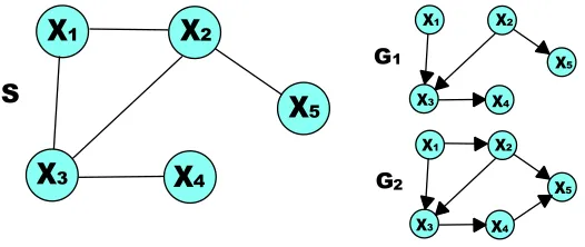
To keep the property that the result of OS converges to the true graph in the sample limit, the constraint should at least authorize the true skeleton. Since knowing the true skeleton is a strong as-sumption and learning it with high confidence from finite data is a hard task, we propose to consider a more flexible constraint than fixing the skeleton. To this end, we introduce a super-structure as:
Definition 4. An undirected graph S= (V,ES)is said to be a super-structure of a DAG G= (V,EG),
if the skeleton of G, G0= (V,EG0) is a subgraph of S (i.e., EG0 ⊆ES). We say that S contains the
skeleton of G.
X
S
G
G
1
X
2X
3X
4X
5X1 X2
X3 X4
X5
1
2
X1 X2
X3 X4
X5
Figure 1: In a search constrained by S, G1could be considered but not G2becausehX4,X5i 6∈ES.
inference from data given a super-structure S: S is assumed to be sound, and the search space is restricted to DAGs whose skeletons are contained in S as illustrated in Figure 1. Actually, the “skeleton” learned by MMPC is used as a super-structure in MMHC. In fact, the skeleton of the graph returned by MMHC is not proven to be the same than the learned one; some edges can be missing. It is the same for the candidate parents in SC. Thus, the idea of super-structure already existed, but we define it explicitly, which has several advantages.
First, a dedicated terminology enables to emphasize two successive and independent phases in structure learning problem: on one hand, learning with high probability a sound super-structure S (sparse if possible); on the other hand, given such structure, searching efficiently the restricted space and returning the best optimum found (global optimum if possible). This problem cutting enables to make clearer the role and effect of each part. For example, since SC and MMHC use the same search, comparing their results allow us directly to evaluate their super-structure learning approach. Moreover, while conceiving a search strategy, it could be of a great use to consider a super-structure given. This way, instead of starting from a general intractable case, we have some framework to assist reasoning: we give some possible directions in our future work. Finally, this manner to apprehend the problem already integrates the idea that the true skeleton will not be given by an IT approach; hence, it could be better to learn a bit denser super-structure to reduce missing edges, which should improve accuracy.
Finally, we should explain how practically a sound super-structure S can be inferred. Even without knowledge about causality, a quick analysis of the system could generate a rough draft by determining which interactions are impossible; localization, nature or temporality of variables often forbid evidently many edges. In addition, for any IT-based technique to learn the skeleton, the neighborhood of variables or their Markov blanket could be used to get a super-structure. This one should become sound while increasing the significance level of the tests: this is because we only need to reduce false negative discovery. Although the method used in PC algorithm could be a good candidate to learn a not sparse but sound super-structure, we illustrate our idea with MMPC in Section 5.1.
4.2 Constraining and Optimizing
From now on, we will assume that we are given a super-structure S= (X,ES)over X. We refer to
the neighborhood of a variable Xi in S by N(Xi), that is, the set of nodes connected to Xi in S (i.e.,
{Xj| hXi,Xji ∈ES}); m is the maximal degree of S, that is, m=maxXi∈X|N(Xi)|. Our task is to
X
S
A
X ,X ,X ,X }
A
X ,X ,X ,X }
1
X
2X
3X
4X
5X
6X
7X1 X2
X3
X6
X7
X1 X2
X3
X6
X5
X4
X4
X5
X7
1
2
1 2 3 4 5
1 3 4 5 7
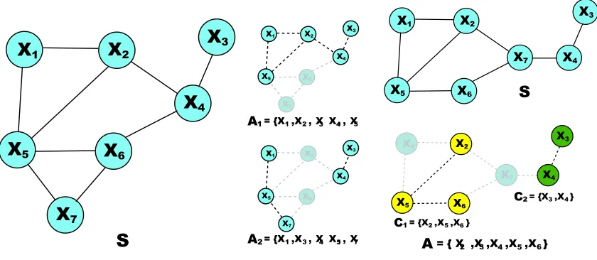
Figure 2: A1 is in Con(S), but not A2 because in SA2, X7
and X4are not connected.
S
X1 X2
X3
X4
X5 X6
X7
X1
X7
X2
X3
X4
X5 X6
A = {X ,X ,X ,X ,X }2 3 4 5 6
C1 2 56
C234
Figure 3: The maximal connected subsets of A: C1 and C2.
Since the parents of every Xiare constrained to be included in N(Xi), the function F has to be
defined only for∀A⊆N(Xi). Consequently, computation of F in step (b) becomes:
(b*) For each Xi∈X and each A⊆N(Xi)
Calculate Fs(Xi,A)and Fp(Xi,A)using (2)
Only the underlined part has been modified; clearly, F still can be computed recursively since
∀Xj ∈A, the subset A\{Xj}is also included in N(Xi), and its F value is already known. With this
slight modification, the time complexity of computing F becomes O(n2m), which is a decisive im-provement opening many perspectives; more details are given at the end of this section. However, to keep formulae (5) and (3) correct, F(Xi,A)for any subset A has to be replaced by F(Xi,A∩N(Xi)).
Before simplifying the calculation of M, it is necessary to introduce the notion of connectivity:
Definition 5. Given an undirected graph S= (X,ES), a subset A⊆X is said to be connected if
A6= /0and the subgraph of S induced by A, SA, is connected (cf. Figure 2).
In our study, connectivity will always refer to the connectivity in the super-structure S. Con(S)
will refer to the set of connected subsets of X. In addition, each not empty subset of X can be broken down uniquely into the following family of connected subsets:
Definition 6. Given an undirected graph S= (X,ES)and a subset A⊆X, let S1= (C1,E1),···,Sp= (Cp,Ep) be the connected components of the induced subgraph SA. The subsets C1,···,Cp are
called the maximal connected subsets of A (cf. Figure 3).
The most important property of the maximal connected subsets C1,···,Cpof a subset A is that,
when p>1 (i.e., when A6∈Con(S)) for any pair Ci, Cj with i6= j, Ci∩Cj= /0 and there is no
edges in S between nodes of Ciand nodes of Cj. Next we show that the value of M for subsets that
of Algorithm 1. The validity of our algorithm is simultaneously proved.
Theorem 2. A constrained optimal graph can be found by computing M only over Con(S).
Proof: First, let consider a subset A6∈Con(S), its maximal connected subsets C1,···,Cp (p>1),
and an optimal constrained DAG G∗= (A,E∗). Since G∗is constrained by the super-structure, and following the definition of the maximal connected subsets, there cannot be edges in G∗between any element in Ci and any element in Cj if i6= j. Therefore, the edges of G∗can be divided in p sets
E=E1∪ ···∪Epwith Gi= (Ci,Ei)a DAG over every Ci. Moreover, all Giare optimal constrained
graphs otherwise G∗would not be. Consequently, we can derive the two following formulas:
Ms(A) = p
∑
i=1Ms(Ci), (7)
Ml(A) =Ml(C1). (8)
Formula (7) directly follows our previous considerations that maximizing the score over A is equiv-alent to maximizing it over each Ciindependently, since they cannot affect each other. Actually, any
Ml(Ci)is an optimal sink and could be selected in (8); we chose Ml(C1)since it is accessed faster
when using the data structure proposed in Section 4.3 for M. By using (7) and (8) the value of M for unconnected subsets can be directly computed if needed from the values of smaller connected subsets. Therefore, we propose to compute M only for connected subsets by replacing step (d) with (d∗) in Algorithm 2 described below. Since each singleton{Xi}is connected, step (c) is not raising
a problem. In step (d∗) we consider A∈Con(S)and apply formula (5), if there is Xj∈A such that
Bj=A\{Xj}is not connected, we then can directly calculate Ms(Bj)by applying (7). the values of
Msfor the maximal connected subsets of Bjare already computed since these subsets are of smaller
sizes than A. Therefore, Ml(A)and Ms(A)can be computed. Finally, it is also possible to retrieve
w∗from (6) by using (8) if T is not connected, which conclude the proof of this Theorem.
We can now formulate our optimized version of Algorithm 1 for optimal DAG search condi-tioned by a super-structure S:
Algorithm 2.
(a*) Initialize∀Xi∈X, Fs(Xi,/0)and Fp(Xi,/0)with (1)
(b*) For each Xi∈X and each A⊆N(Xi)
Calculate Fs(Xi,A)and Fp(Xi,A)using (2)
(c*) Initialize∀Xi, Ms({Xi})and Ml({Xi})using (4)
(d*) For each A∈Con(S)with|A|>1
Calculate Ms(A)and Ml(A)using (5) and(7)
(e*) Build an optimal ordering w∗using (6) and(8)
(f*) Return the best w∗-linear graph G∗w∗ using (3)
once, the total computational complexity is in O(n2m+|Con(S)|); here again complexity refers to the number of times formulae (2) or (5) are computed. We will describe in the next Section a method to consider only connected subsets, and come over the number of connected subsets of S in Section 4.4. Although set operators are used heavily in our algorithm, such operations can be efficiently implemented and considered of a negligible cost as compared to other operations, such as score cal-culations. Concerning the complexity of calculating F, O(n2m)is in fact a large upper bound. Still, since it depends only linearly on the size of the graphs, F can be computed for graphs of any size if their maximal degree is less than around thirty. This enables usage of this function in new search strategies for many real systems that could not be considered without constraint. We should remark that some cases of interest still cannot be studied since this upper limitation on m constrains also the maximal number of children of every variables. However, this difficulty concerns also many IT-approaches since their complexity also depends exponentially on m (see Tsamardinos et al. 2006 for MMPC and Kalisch and B ¨uhlmann 2007 for PC). Finally, like in Algorithm 1, the number of scores calculated can be reduced to O(nmc)by constraining on the number of parents.
Although the number of M and F values calculated is strictly reduced, a potential drawback of Algorithm 2 is that memory cannot be recycled anymore. First, when (5) is used during step (d∗), now Fs(Xi,Bj∩N(Xi))is required, and nothing can be said about |Bj∩N(Xi)|implying that
we should store every value of Fs computed before. Similar arguments hold for Fp in case Ml is
used to store optimal graphs, and for Msand Ml because (7) and (8) could have to be used anytime
during (d∗) and (e∗) respectively. However, since space complexity of F is O(n2m) and the one of M is O(|Con(S)|)(cf. next section), if m is bounded Algorithm 2 should use less memory than Algorithm 1 even when recycling memory (i.e., O(√n2n) assuming that a set takes O(1) space). This soften the significance of recycling memory in our case.
Finally, since our presentation of Algorithm 2 is mainly formal, we should detail how it is practically possible to browse efficiently only the connected subsets of X. For this, we present in the next section a simple data structure to store values of M and a method to build it.
4.3 Representation of Con(S)
For every A∈Con(S)we define N(A) = S
Xi∈AN(Xi)
\A, that is the set of variables neighboring A in S. For every Xi6∈A, we note A+i =A∪ {Xi}, it is connected if and only if Xi∈N(A). Finally,
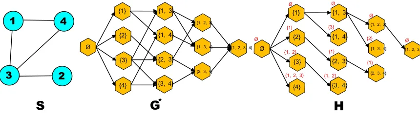
for a subset A not empty, let min(A) be the smallest index in A, that is, min(A) =i means that Xi∈A and ∀Xj ∈A, j≥i; by convention, min(/0) =0. Now we introduce an auxiliary directed
graph G?= (Con(S)?,E?), where Con(S)?=Con(S)∪ {/0}and the set of directed edges E?is such
that there is an edge from A to B if and only if A⊂B and |B|=|A|+1. In other words, with the convention that N(/0) =X, E?={(A
,A+i ),∀A∈Con(S)?and∀Xi ∈N(A)}. Actually, G? is
trivially a DAG since arcs always go from smaller to bigger subsets. Finally, let define H as being the spanning tree obtained from the following depth-first-search (DFS) on G?:
• The search starts from /0.
• While visiting A∈Con(S)?: for all X
ki ∈N(A)considered by increasing indices (i.e., such
that k1<···<kp, where p=|N(A)|) visit the child A+ki if it was not yet done. When all
children are done, the search backtracks.
1 4
3 2
S
{1}
{2}
{3}
{4}
{1,3}
{1,4}
{2,3}
{3,4}
{1,2,3}
{1,3,4}
{2,3,4}
{1,2,3,4}
H
Ø{1}
{2}
{3}
{4}
{1,3}
{1,4}
{2,3}
{3,4}
{1,2,3}
{1,3,4}
{2,3,4}
{1,2,3,4} Ø
G
{3}
{2} {1}
Ø
Ø Ø
Ø
Ø {1}
{1} {1,2}
{1,2} {1,2,3}
Figure 4: G?and H for a given S. Fb(A)is indicated in red above each node in H.
Algorithm 2; this structure is illustrated by an example in Figure 4. Further, we propose a method to build H directly from S without having to build G?explicitly. First, we notice that after visiting A,
every B∈Con(S)such that B⊃A have been visited for sure. When visiting A, we should consider only the children of A that were not yet visited. For this, we define:
• Fb(A)is the set of forbidden variables of A, that is: for every B∈Con(S)with B⊃A, B has been already visited if and only if B⊇A+j with Xj∈Fb(A).
By defining recursively this forbidden set for every child of A that has not yet been visited, we derive the following method to build H:
Method 1.
1: Create the root of H (i.e., /0), and initialize Fb(/0) =/0. 2: For i from 0 to n−1, and for all A in H such that|A|=i 3: Set Fb∗=Fb(A),
4: For every Xkj ∈N(A)\Fb(A)considered by increasing indices
5: Add to A the child A+k
j in H and define Fb(A
+
kj) =Fb
∗
6: Update Fb∗=Fb∗k+
j
The correctness of Method 1 is proven in the next Theorem. In order to derive the time com-plexity of step (d∗) in terms of basic operations, while using Method 1 in Algorithm 2, let consider that the calculation takes place on a x-bit machine and that n is at maximum few times greater than x. Thus, subsets requires O(1)space, and any operations on subsets are done in O(1)time, except min(A)(in O(log(n))time).
Theorem 3. The function M can be computed in time and space proportional to O(|Con(S)|), up to some polynomial factors. With Method 1, M is computed in O(log(n)n2|Con(S)|)time and requires O(|Con(S)|)space.
Proof: First, to prove correctness of Method 1, we show that if Fb(A)is correctly defined in regard to our DFS, the search from A proceeds as expected and that before back tracking every connected superset of A has been visited. The case when all the variables neighboring A are forbidden being trivial, we directly consider all the elements Xk1,···,Xkp of N(A)\Fb(A) by increasing indices
like in DFS (with p≥1). Then, A+k
1 should be visited first, and Fb(A
+
Fb(A) among the supersets of A+j there is also the supersets of A++k
1,j. Now let suppose that the
forbidden sets were correctly defined and that the visits correctly proceeded until A+k
i: if i=p by
hypothesis we explored every connected supersets of the children of A and the search back track correctly. Otherwise, we should define Fb(A+k
i+1) =Fb(A)∪ {Xk1} ∪ ··· ∪ {Xki}=Fb(A
+
ki)
+
ki to take
into account all supersets visited during the previous recursive searches. Although Method 1 does not proceed recursively (to follow the definition of M), since it uses the same formulae to define the forbidden sets, and since Fb(/0)is correctly initialized, H is built as expected.
To be able to access easily M(A), we keep for every node an auxiliary set defined by Nb(A) = N(A)\Fb(A)that is easily computed as processing Method 1. Since there is O(|Con(S)|) nodes in H, each storing a value of M and two subsets requiring O(1) space, the assertion about space complexity is correct.
Finally, building a node requires O(1)set operations. To access M(A)even for an unconnected subset, we proceed on the following manner: we start from the root, and define T=A. Then, when we rushed the node B⊆A, with i=min(Nb(B)∩T), we withdraw Xifrom T, and go down to the
ithchild of B. If i=0 then if T= /0we found the node of A; otherwise we rushed the first maximal connected component of A, that is, C1of which we can accumulate the M value in order to apply (7) or (8). In that case, we continue the search by restarting from the root with the variables remaining in T. In any cases, at maximum min is used O(n)times to find M(A), implying a time complexity of O(log(n)n2)for formula (5).
It is interesting to notice that, even without memoization, the values of M can be calculated in different order. For example, by calling Hi the subtree of H starting from{Xi}, only values of
M over Hj such that j≥i are required. Then it is feasible to calculate M from Hn to H1, which could be used to apply some branch-pruning rules based on known values of M or to apply different strategies depending on the topology of the connected subset; these are only suppositions.
More practically, other approach could be proposed to build a spanning tree of G?and Method
1 is presented here only to complete our implementation and illustrate Theorem 3. We should note that one can also implement the calculation of M over Con(S)in a top-down fashion using memo-ization and an auxiliary function to list maximal connected components of a subset. However, such implementations will be less efficient both in space and time complexity. Even without considering the cost of recursive programming, listing connected components is in O(nm). Then, in order to not waste an exponential factor of memory, self balanced trees should be used to store the memorized values of M: it would require O(n) time to access a value and up to O(n2) if (7) is used. This should be repeated O(n)times to apply (5), which implies a complexity of around O(n3|Con(S)|). Consequently, we believe that Method 1 is a competitive implementation of step (d∗).
4.4 Counting Connected Subsets of a Graph
To understand the complexity of Algorithm 2, the asymptotic behavior of |Con(S)| should be derived, depending on some attributes of S. Comparing the trivial cases of a linear graph (i.e., m≤2) where|Con(S)|=O(n2)and a star graph (i.e., one node is the neighbor of all others) where
|Con(S)|=2n−1+n−1 clearly indicates that|Con(S)|depends strongly on the degrees of Srather than on the number of edges or number of cycles. One important result from Bj ¨orklund et al. (2008) is that|Con(S)|=O(βn
m)withβm= (2m+1−1)
1
m+1 a coefficient that only depends on the maximal
5 10 15 20 25 30 35 1 .7 5 1 .8 5 1 .9 5 (a)
n
γm(
n)
m 3 4 5 6γ3=1.81…
γ4=1.92…
γ5=1.96…
20 40 60 80 100
1 .0 1 .4 1 .8 (b)
n
δm~(
n)
m~ 0.1 0.5 0.8 1 1.5 1.9 2 2.3 2.8 3 3.50.5 1.0 1.5 2.0 2.5 3.0 3.5
1 .0 1 .4 1 .8 (c) m~ δm~
0.5 1.0 1.5 2.0 2.5 3.0 3.5
0 1 0 0 3 0 0 5 0 0 (d) m~ m a x im a l g ra p h s iz e in a v e ra g e
w ith nmax(O S)=30
Coeffi cient of upper complexity for various m Coeffi cient of average complexity for various m~
Behaviour of δm D epending on m~ ~ ~n for a constrained O S given mmax ~
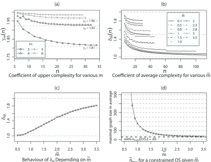
Figure 5: Experimental derivation ofγm,δm˜ and ˜nmax2(m˜).
Still, since this upper bound is probably over-estimated, we tried to evaluate a better one exper-imentally. For every pair(m,n)of parameters considered , we randomly generated 500 undirected graphs S pushing their structures towards a maximization of the number of connected subsets. For this, all the nodes had exactly m neighbors and S should at least be connected. Then, since after a first series of experiments the most complex structures appeared to be similar to full(m−1)-trees, with a root having m children and leaves being connected to each other, only such structures were considered during a second series of experiments. Finally, for each pair(m,n), from the maximal number Rn,mof connected subsets found, we calculated exp(ln(Rnn,m)))in order to search for an
ex-ponential behavior as shown in Figure 5(a).
Results 1. Our experimental measures led us to propose that|Con(S)|=O(γmn)(cf. Figure 5(a)).
The weak point of our strategy is that more graphs should be consider while increasing n, since the number of possible graphs also increases. Unfortunately, this is hardly feasible in practice since counting gets longer with larger graphs. Nevertheless, Results 1 were confirmed during a more detailed study of the case m=3 using 10 times more graphs and up to n=30. In addition, even this estimated upper bound is practically of a limited interest since it still dramatically overestimates
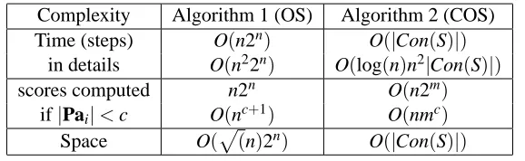
Complexity Algorithm 1 (OS) Algorithm 2 (COS) Time (steps) O(n2n) O(|Con(S)|)
in details O(n22n) O(log(n)n2|Con(S)|)
scores computed n2n O(n2m)
if|Pai|<c O(nc+1) O(nmc)
Space O(p
(n)2n) O(|Con(S)|)
Table 1: Improvement achieved by COS.
S |Con(S)| some values Tree-like O(αn
m) α3≈1.58,α4≈1.65,α5≈1.707
General O(βn
m) β3≈1.968,β4≈1.987,β5≈1.995
Measured O(γn
m) γ3≈1.81,γ4≈1.92,γ5≈1.96
In average O(δn
˜
m) δ1.5≈1.3,δ2≈1.5,δ2.5≈1.63,δ3≈1.74 Table 2: Results on|Con(S)|
the ones used in previous experiments. To illustrate that O(γmn) is a pessimistic upper bound, we
derived the theoretical upper bound of|Con(S)|for tree-like structures of maximal degree m. This is given as an example, although it might help estimation of|Con(S)|for structures having a bounded number of cycles. The proof is deferred to the Appendix.
Proposition 1. If S is a forest, then|Con(S)|=O(αn
m)withαm= (2
m−1+1
2 )
1
m−1.
Finally, we studied the average size of|Con(S)|for a large range of average degrees ˜m. For each pair(n,m˜)considered, we generated 10000 random graphs and averaged the number of connected subsets to obtain Rn,m˜. No constraint was imposed on m, since graphs were generated by randomly adding edges untilbn ˜2mc. In each case, we calculated exp(ln(Rn,m˜)
n ))to search for an asymptotic
be-havior on ˜m.
Results 2. On average, for super-structures having an average degree of ˜m, |Con(S)|increases asymptotically as O(δm˜n), see Figure 5(b) and (c) for more details.
Based on the assumption that Algorithm 1 is feasible at maximum for graphs of size nmax1=30
(Silander and Myllym¨aki, 2006), we calculated ˜nmax2(m˜) =nmax1
ln(2)
ln(δm˜)that can be interpreted as an
estimation of the maximal size of graphs that can be considered by Algorithm 2 depending on ˜m. As shown in Figure 5(d), on average, it should be feasible to consider graphs having up to 50 nodes with Algorithm 2 if ˜m=2. Moreover, since lim
˜
m→0δm˜ =1, our algorithm can be applied to graphs of any sizes if they are enough sparse. Unfortunately, the case when ˜m<2 is not really interesting
since it implies that networks are mainly unconnected.
expo-nentially with n. Moreover, our algorithm can be applied to some small real networks that are not feasible for Algorithm 1.
5. Experimental Evaluation
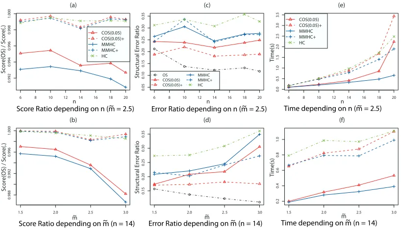
Although the demonstrations concerning correctness and complexity of Algorithm 2 enable us to anticipate results obtained experimentally, some essential points remain to be studied. Among them, we should demonstrate practically that, in the absence of prior knowledge, it is feasible to learn a sound super-structure with a relaxed IT approach. We choose to test our proposition on MMPC (Tsamardinos et al., 2006) in Section 5.2; the details of this algorithm are briefly reintroduced in Section 5.1.4. Secondly, we compare COS to OS to confirm the speed improvement of our method and study the effect of using a sound constraint in Section 5.3. We also should evaluate the worsening in terms of accuracy due to the incompleteness of an approximated super-structure. In this case we propose and evaluate a greedy method, COS+, to improve substantially the results of COS. In Section 5.4, we compare our methods to other greedy algorithms to show that, even with an incomplete super-structure, COS, and especially COS+, are competitive algorithms to study small networks. Finally we illustrate this point by studying the ALARM Network (Beinlich et al., 1989) in Section 5.5, a benchmark of structure learning algorithm for which OS is not feasible.
5.1 Experimental Approach
Except in the last real experiment, we are interested in comparing methods or algorithms for various set of parameters, such as: the size of the networks n, their average degree ˜m (to measure effect of sparseness on Algorithm 2), the size of data considered d and the significance levelαused to learn the super-structure.
5.1.1 NETWORKS ANDDATACONSIDERED
Due to the size limitation imposed by Algorithm 1, only small networks can be learned. Further, since there it is hardly feasible to find many real networks for every pair (n,m˜) of interest, we randomly generated the networks to which we apply structure learning. Given a pair(n,m˜), DAGs
of size n are generated by adding randomlybn ˜2mcedges while assuring that cycles are not created. For simplicity, we considered only Boolean variables; therefore, Bayesian networks are ob-tained from each DAG by generating conditional probabilities P(Xi=0|Pai=paki) for all Xi and
all possible paki by choosing a random real number in]0,1[. Then, d data are artificially generated from such Bayesian networks, by following their entailed probability distribution.
Finally, the data are used to learn a network with every algorithm and some criteria are mea-sured. In order to generalize our results, we repeat g times the previous steps for each quadruplet
(n,m˜,α,d). The values of each criterion of comparison for every algorithm are averaged on the g learned graphs.
5.1.2 COMPARISONCRITERIA
n or ˜m in a diagram, we do not directly represent scores (their values change radically for different parameters) but use a score ratio to the optimal score: Score(GOS)
Score(GOther), where the label of the graph
indi-cates which Algorithm was used. The better is the score obtained by an algorithm, the closer to 1 is its score ratio. We preferred to use the best score rather than the score of the true network, because the true network is rarely optimal; its score is even strongly penalized if its structure is dense and data sets are small. Therefore, it is not convenient to use it as a reference in terms of score.
The second criterion is a measure of the complexity estimated by the execution time of each algorithm, referred as Time. Of course, this is not the most reliable way to estimate complexity, but since calculations are done on the same machine, and since measures are averaged on few similar calculations, execution time should approximate correctly the complexity. To avoid bias of this criterion, common routines are shared among algorithms (such as the score function, the structure learning method and the hill climbing search).
Finally, since our aim is to learn a true network, we use a structural hamming distance that compares the learned graph with the original one. As proposed in Tsamardinos et al. (2006), to take into consideration equivalence classes, the CPDAGs of both original and learned DAGs are built and compared. This defines the structural error ratio SER of a learned graph, which is the number of extra, missing, and wrongly oriented edges divided by the total number of edges in the original graph. In our case, we penalize wrongly oriented edges only by half, because we consider that errors in the skeleton are more “grave” than those in edges orientation. The reason is not only visual: a missing edge, or an extra edge, implies more mistakes in terms of conditional independencies in general than wrongly oriented ones. Moreover, in CPDAGs, the fact that an edge is not correctly oriented is often caused by extra or missing edges. Furthermore, such a modification does not intrinsically change the results, since it benefits every algorithm on the same manner.
5.1.3 HILLCLIMBING
Although hill climbing searches are used by different algorithms, we implemented only one search that is used in all cases. This search can consider a structural constraint S, and is given a graph Ginit from which to start the search. Then it processes as summarized in Section 2.2, selecting at each step the best transformation among all edge withdrawals, edge reversals and edge additions according to the structure constraint. The search stops as soons as the score cannot be strictly improved anymore. If several transformations involve the same increase of the score, the first transformation encountered is applyed. This implies that the results will depend on the ordering of the variables; however, since the graphs considered are randomly generated, their topological ordering is also random, and in average the results found by our search should not be biased.
5.1.4 RECALL ONMMPC
In Section 5.3 a true super-structure is given as a prior knowledge; otherwise we should use an IT-approach to approximate the structural constraint S from data. Since MMHC algorithm is included in our experiments, we decided to illustrate our idea of relaxed independency testing on MMPC strategy (Tsamardinos et al., 2006).
In MMPC, the following independency test is used to infer independencies among variables. Given two variables Xi and Xj, it is possible to measure if they are independent conditioning on a
subsets of variables A⊆X\{Xi,Xj}by using the G2 statistic (Spirtes et al., 2000), under the null
Xi=a, Xj=b and A=c simultaneously in the data, G2is defined by:
G2=2
∑
a,b,c Nabcln
NabcNc NacNbc
.
The G2 statistic is asymptotically distributed as χ2 under the null hypothesis. Theχ2 test returns a p-value, PIT(Xi,Xj|A), that corresponds to the probability of falsely rejecting the null hypothesis
given it is true; in MMPC, the effective number of parameters defined in Steck and Jaakkola (2002) is used as degree of freedom. Thus given a significance levelα, if PIT≤αnull hypothesis is rejected,
that is, Xi and Xj are considered as conditionally dependent. Otherwise, the hypothesis is accepted
(abusing somehow of the meaning of the test), and variables are declared conditionally independent. The main idea of MMPC is: given a conditioning set A, instead of considering only PIT(Xi,Xj|A)to
decide dependency, it is more robust to consider max
B⊆APIT(Xi,Xj|B); that way, the decision is based
on more tests; p-values already computed are cached and reused to calculate this maximal p-value. Finally, MMPC build the neighborhood of each variable Xi(called the set of parents and children, or
PC) by adding successively potential neighbors of Xi from a temporary set T. While conditioning
on the actual neighborhood PC, the variable Xk ∈T that minimizes the maximal p-value defined
before is selected because it is the variable the most related to Xi. During this phase, every variable
that appears independent of Xiis not considered anymore and withdrawn from T. Then when Xkis
added to PC, we test if all neighbors are always conditionally dependent: if some are not, they are withdrawn from PC and not considered anymore. This process ends when T becomes empty.
We present further the details of our implementation of MMPC, referred as Method 2; it is slightly different from the original presentation of MMPC, but the main steps of the algorithm are the same. One can prove by using Theorem 1 that if the independencies are correctly estimated, this Method should return the true skeleton, which should be the case in the sample limit. About compu-tational complexity, one can derive that MMPC should calculate around O(n22m)tests in average. However, nothing can be said in practice about the maximal size of PC, especially if many false dependencies occurs. Therefore, the time complexity of MMPC can be in the worst case O(n22n).
Method 2 (MMPC). (Tsamardinos et al., 2006) 1: For∀Xi∈X
2: Initialize PC=/0and T=X\ {Xi}
3: While T6= /0
4: For∀Xj∈T, if max
B⊆PCPIT(Xi,Xj|B)>αthen T=T\{Xj}
5: Define Xk=min Xj∈T
max
B⊆PCPIT(Xi,Xj|B)and PC=PC∪ {Xk}
6: For∀Xj∈PC\{Xk}, if max B⊆PC\{Xj}
PIT(Xi,Xj|B)>αThen PC=PC\{Xj}
7: N(Xi) =PC
8: For∀Xi∈X and∀Xj∈N(Xi)
9: If Xi6∈N(Xj)Then N(Xi) =N(Xi)\{Xj}
5.2 Learning a Super-structure with MMPC
0
.0
0
.4
0
.8
1
.2
(a)
α
R
a
ti
o
Error − M issing d= 10000 d= 5000 d= 500
d= 10000 d= 5000 d= 500
0 1e− 10 1e− 7 1e− 4 0.01 0.05 0.1 0.25 0.5
0
5
1
5
2
5
(b)
α
T
im
e
(
s)
Tim e d= 10000 d= 5000 d= 500
0 1e− 10 1e− 7 1e− 4 0.01 0.05 0.1 0.25 0.5
Error and M issing Ratio depending on α (n = 50, m = 2.5)~ Tim e of M M PC depending on α (n = 50, m = 2.5)~
Figure 6: Effects of d andαon the results of Method 2.
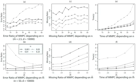
before, we average our criteria of interest over g=50 different graphs for every set of parameters. In the present case our criteria are: the time of execution Time, the ratio of wrong edges (missing and extra) Error, and the ratio of missing edges Miss of the learned skeleton. Here again, these ratios are defined while comparing to the true skeleton and dividing by its total number of edges
bn ˜m
2 c. While learning a skeleton, Error should be minimized; however in the case of learning a super-structure, Miss is the criterion to minimize.
Results 3 limα→1Miss(α) =0, which validates our proposition of using higherα to learn super-structures (cf. Figure 6(a)). Of course, we obtain the same results with increasing data, limd→∞Miss(α) =0. However, since whenα→1, Time(α)≈O(n22n−2), high values ofαcan be
practically infeasible (cf. Figure 6(b)). Therefore, to escape a time-consuming structure-learning phase,αshould be kept under 0.25 if using MMPC.
In Figure 6(a), one can also notice that Error is minimized forα≈0.01, that is why such values are used while learning a skeleton. Next, we summarize the effect of n and ˜m on the criteria:
Results 4 Increasingαimproves uniformly the ration of missing edges independently of n and ˜m (cf. Figure 7(c) and (d)). Miss(α)is not strongly affected by increasing n but it is by increasing ˜m; thus for dense graphs, the super-structures approximated by MMPC will probably not be sound.
Previous statement could be explained by the fact that when ˜m increases, the size of conditional probability tables of each node increases enormously. Thus, the probability of creating weak or nearly unfaithful dependencies between a node and some of its parents also increases. Therefore, the proportion of edges that are difficult to learn increases as well. To complete analysis of Figure 7, we can notice as expected that Time increases on a polynomial manner with n (cf. Figure 7 (e)), which penalizes especially the usage of highα. Error(α)is minimized in general forα=0.01 or α=0.05 depending on n and ˜m: for a given ˜m, lowerα(such asα=0.01) are better choices when
n increases (cf. Figure 7(a)); conversely, if ˜m increases for a fixed n, higherα(such asα=0.05) are favored (Figure 7(b)). This can be justified, since if ˜m is relatively high, higherαthat are more permissive in terms of dependencies will miss less edges, as opposed to lower ones with finite set of data.
In conclusion, although α≈0.01 is preferable while learning a skeleton with MMPC, higher