Learning Sparse Representations by Non-Negative Matrix Factorization and Sequential Cone Programming

Learning Sparse Representations by

Non-Negative Matrix Factorization and

Sequential Cone Programming

Matthias Heiler [email protected]

Christoph Schn¨orr [email protected]

Computer Vision, Graphics, and Pattern Recognition Group Department of Mathematics and Computer Science

University of Mannheim D-68131 Mannheim, Germany

Editors: Kristin P. Bennett and Emilio Parrado-Hern´andez

Abstract

We exploit the biconvex nature of the Euclidean non-negative matrix factorization (NMF) optimiza-tion problem to derive optimizaoptimiza-tion schemes based on sequential quadratic and second order cone programming. We show that for ordinary NMF, our approach performs as well as existing state-of-the-art algorithms, while for sparsity-constrained NMF, as recently proposed by P. O. Hoyer in

JMLR 5 (2004), it outperforms previous methods. In addition, we show how to extend NMF

learn-ing within the same optimization framework in order to make use of class membership information in supervised learning problems.

Keywords: non-negative matrix factorization, second-order cone programming, sequential convex optimization, reverse-convex programming, sparsity

1. Introduction

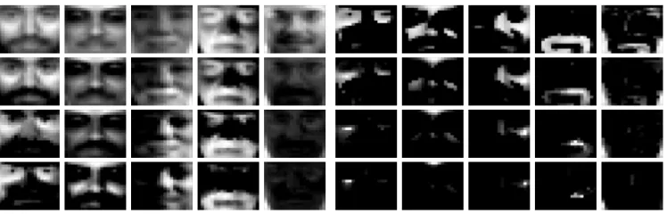
Originally proposed to model physical and chemical processes (Shen and Isra¨el, 1989; Paatero and Tapper, 1994), non-negative matrix factorization (NMF) has become increasingly popular for feature extraction in machine learning, computer vision, and signal processing (e.g., Hoyer and Hyv¨arinen, 2002; Xu et al., 2003; Smaragdis and Brown, 2003). One reason for this popularity is that NMF codes naturally favor sparse, parts-based representations (Lee and Seung, 1999; Donoho and Stodden, 2004) which in the context of recognition can be more robust than non-sparse, global features. In some application domains, researchers suggested various extensions of NMF in order to enforce very localized representations (Li et al., 2001; Hoyer, 2002; Wang et al., 2004; Chi-chocki et al., 2006). For example, Hoyer (2004) recently proposed NMF subject to additional con-straints that allow particularly accurate control over sparseness and, indirectly, over the localization of features—see Figure 1 for an illustration.

Figure 1: Motivation of NMF with sparseness constraints. Five basis functions (columns) with sparseness constraints ranging from 0.1 (first row, left) to 0.8 (last row, right) on W were trained on the CBCL face database. A moderate amount of sparseness encourages local-ized, visually meaningful base functions.

that for ordinary NMF our schemes perform as well as existing state-of-the-art algorithms, while for sparsity-constrained NMF they outperform previous methods. In addition, our approach easily extends to supervised settings similar to Fisher-NMF (Wang et al., 2004).

Organization. In Section 2, we introduce various versions of the NMF optimization problem.

Then, we first consider the unconstrained case in Section 3. The representation of the sparsity constraints and the corresponding optimality conditions are described in Section 4. Using convex optimization problems as basic components, we suggest algorithms for solving the general NMF problem in Section 5. Numerical experiments validate our approach in Section 6. We conclude in Section 7.

Notation. For any m_×n-matrix A, we denote columns by A= (A_•1, . . . ,A•n) and rows by

A= (A1_•, . . . ,Am_•)⊤. V ∈Rm+×n is a non-negative matrix of n data samples, and W ∈Rm+×r a

corresponding basis with loadings H_∈Rr+×n. Furthermore, we denote by e the column vector with

all entries set to 1. _kx_kp represents theℓp-norm for vectors x, kxkp= (∑i|xi|p)1/p, andkAkF the

Frobenius norm for matrices A: _kA_k2_F =∑i,jA2i j=tr(A⊤A). vec(A) = (A⊤_•1, . . . ,A⊤•n)⊤is the vector

obtained by concatenating the columns of the matrix A. The Kronecker product of two matrices A and B is written A⊗B (see, e.g., Graham, 1981). As usual, relations between vectors and matrices,

like x_≥0,A_≥0, are understood elementwise.

2. Variations of the NMF Optimization Problem

2.1 Unconstrained NMF

The original NMF problem reads with a non-negative matrix of n data samples V _∈Rm+×n, a matrix

of basis functions W _∈Rm+×r, and corresponding loadings H∈Rr+×n:

min

W,H kV−W Hk 2 F

s.t. 0_≤W,H.

(1)

This problem is non-convex. There are algorithms that compute the global optimum for such prob-lems (Floudas and Visweswaran, 1993), however, they do not yet scale up to the large probprob-lems common in, e.g., machine learning, computer vision, or engineering. As a result, we will con-fine ourselves to efficiently compute a local optimum by solving a sequence of convex programs (Section 3.2).

2.2 Sparsity-Constrained NMF

Although NMF codes tend to be sparse (Lee and Seung, 1999), it has been suggested to control sparsity by more direct means. A particularly attractive solution was proposed by Hoyer (2004) where the following sparseness measure for vectors x_∈Rn+, x6=0, was used:

sp(x):=√ 1 n₋1

_√

n₋kxk1 kx_k2

. (2)

Because of the relations

1

√_nkx_k1≤ kxk2≤ kxk1, (3)

the latter being a consequence of the Cauchy-Schwarz inequality, this sparseness measure is bounded:

0_≤sp(x)_≤1. (4)

The bounds are attained for minimal sparse vectors with equal non-zero components where sp(x) = 0 and for maximal sparse vectors with all but one vanishing components where sp(x) =1. These bounds are useful from a practical viewpoint since they make it relatively intuitive to estimate sparseness for a given vector x. In addition, we found that (2) can conveniently be represented in terms of second order cones (Section 4), allowing efficient numerical solvers to be applied.

In this text, we will sometimes write sp(M)_∈Rn, meaning sp(_·) is applied to each column of matrix M_∈Rm×n and the results are stacked in a column vector. Using this convention, the following constrained NMF problem was proposed in (Hoyer, 2004):

min

W,H kV−W Hk 2 F

s.t. 0_≤W,H

sp(W) =sw

sp(H⊤) =sh,

(5)

where sw,share user parameters. The sparsity constraints control (i) to what extent basis functions

of the data V . In a pattern recognition application the sparsity constraints effectively weight the desired generality over the specificity of the basis functions.

Instead of using equality constraints we will slightly generalize the constraints in this work to intervals smin_{w ≤}sp(W)_≤smax_w and smin_{h ≤}sp(H⊤)_≤smax_h . This disburdens the user from choosing exact parameter values sw,sh, which can be difficult to find in realistic scenarios. In particular, it

allows for smax_h =smax_w =1, which may often be useful.

Consequently, we define the sparsity-constrained NMF problem as follows:

min

0≤W,H kV−W Hk 2 F

s.t. smin_{w ≤}sp(W)_≤smax_w smin_{h ≤}sp(H⊤)_≤smax_h ,

(6)

where smin_w ,smax_w ,smin_h ,smax_h are user parameters. See Figure 1 and Section 6 for illustrations. Efficient algorithms for solving (6) are developed in Section 5.

2.3 Supervised NMF

When NMF bases are used for recognition, it can be beneficial to introduce information about class membership in the training process. Doing so encourages NMF codes that not only describe the input data well, but also allow for good discrimination in a subsequent classification stage. We propose a formulation, similar to Fisher-NMF (Wang et al., 2004), that leads to particularly efficient algorithms in the training stage.

The basic idea is to restrict, for each class i and for each of its vectors j, the coefficients Hj•to

a cone around the class center µiwhich is implicitly computed in the optimization process:

min

W,H kV−W Hk 2 F

s.t. 0_≤W,H

kµi−Hj•k2≤λkµik1 ∀i,∀j∈class(i).

(7)

As will be explained in Section 5.4, these additional constraints are no more difficult from the view-point of optimization than are the previously introduced constraints in (6). On the other hand, they offer greatly increased classification performance for some problems (Section 6). Of course, if the application suggests, supervised NMF (7) can be conducted with the additional sparsity constraints from (6).

2.4 Assumptions

Throughout the remainder of this paper, the following assumptions are made:

1. The matrices W⊤W and HH⊤ are positive definite.

2. smin_h <smax_h and smin_w <smax_w in (6).

3. The min-sparsity constraints in (6) are essential in the sense that each global optimum of the problem with min-sparsity constraints removed violates at least one such constraint on W and

The first assumption is introduced to simplify reasoning about convergence. In applications, it will regularly be satisfied as long as the number of basis functions r does not exceed size or dimension of the training data: r_≤m,n. Assumption two has been discussed above in connection with (6).

Finally, assumption three is natural, because without the min-sparsity constraint problem (6) would essentially correspond to (1) which is less involved.

3. Solving Unconstrained NMF Problems

We introduced various forms of the NMF problem in the previous section. Next, we concentrate on practical algorithms to find locally optimal solutions. Unlike previous work, where variations of the gradient descent scheme were applied (Paatero, 1997; Hoyer, 2004), our algorithms’ basic building blocks are convex programs for which fast and robust solvers exist. As a side effect, we avoid introducing additional optimization parameters like step-sizes or damping-constants, which is convenient for the user and increases robustness. As a result, just like with Lee and Seung’s fast NMF algorithm (Lee and Seung, 2000), there is no artificial step size parameter to be determined, removing a potential source of errors and inefficiencies.

We next recall briefly the definition of quadratic programs, and then explain our approach to unconstrained NMF. Comparisons to existing work are reported in Section 6.

3.1 Convex Quadratic Programs (QP)

Convex quadratic programs (QP) are optimization problems involving convex quadratic objectives

functions and linear constraints. In connection with unconstrained NMF (1), the QPs to be defined in the next section take the following general form:

min

x

1 2x

⊤_Ax−b⊤_{x, 0≤x, A positive semidefinite. (8)}

We denote the quadratic program (8) with parameters A,b:

QP(A,b) (9)

Note, that for QPs efficient and robust algorithms exist (e.g., Wright, 1996) and software for large-scale problems is available.

3.2 NMF by Quadratic Programming

The unconstrained NMF problem (1) reads:

min

W,H kV−W Hk 2 F

s.t. 0_≤W,H.

Let us fix W and expand the objective function:

kV₋W H_k2_F=tr(V₋W H)⊤(V₋W H)

Algorithm 3.1 QP-based NMF algorithm in pseudocode.

1: initialize W0,H0_≥0 randomly, k_←0

2: repeat

3: Hk+1_←QP-result(Wk,V)using eqn. (10)

4: Wk+1_←QP-result(Hk+1,V)using eqn. (12)

5: k_←k+1

6: untilkV−Wk−1Hk−1k − kV−WkHkk ≤ε

Together with the non-negativity constraints 0_≤H, this amounts to solving the QPs:

QP(W⊤W,W⊤V_•i), i=1, . . .n, (10)

for H_•1, . . . ,H•n. Conversely, fixing H we obtain:

kV₋W H_k2_F=tr(W HH⊤W⊤)₋2tr(V H⊤W⊤) +tr(V⊤V), (11) which amounts to solve the QPs:

QP(HH⊤,HVi•), i=1, . . . ,m, (12)

for W1•, . . . ,Wm•.

We emphasize that by using a batch-processing scheme problems of almost arbitrary size can be handled: The only hard limitation is the number of basis vectors r; the dimension of the basis vectors m can, in principle, grow almost arbitrarily large. This is particularly important for image processing applications where m represents the number of pixels which can be large.

The algorithm is summarized in Alg. 3.1. Note, that the same target function (1) is optimized alternately with respect to H and W . As a result, the algorithm performs a block coordinate descent (cf. Bertsekas, 1999). Furthermore, we may assume that the QPs in (10) and (12) are strictly convex, because typically r_≪m,n (c.f. Section 2.4).

Proposition 1 Under the assumptions of Section 2.4, the algorithm stated in Alg. 3.1 converges to a local minimum of problem (1).

Proof See Bertsekas (1999), Prop. 2.7.1.

4. Sparsity Constraints and Optimality

In this section we develop a geometric formulation of problem (6) in terms of second order cones that fits into the framework of reverse-convex programming (Section 5.1). We note that from the viewpoint of optimization problem (6) is considerably more involved than (1) because the lower sparsity bound imposed in terms of smin_w , smin_h destroys convexity.

4.1 Second Order Cone Programms (SOCP) and Sparsity

The second order cone

L

L

x t

= (x1, . . . ,xn,t)⊤

kxk2≤t

The problem of minimizing a linear objective function, subject to the constraints that several affine functions of the variables are required to lie in

L

min

x∈Rn f

⊤_x

s.t.

Aix+bi c⊤_i x+di

∈

L

Note, that efficient and robust solvers for solving SOCPs exist in software (Sturm, 2001; Mittel-mann, 2003; Mosek 2005). Furthermore, additional linear constraints and, in particular, the condi-tion x_∈Rn+are admissible, as they are special cases of constraints of the form (14). Our approach

to sparsity-constrained NMF, to be developed below, is based on this class of convex optimization problems.

Motivated by the sparseness measure (2) and our goal to compute non-negative representations, we consider the family of convex sets parametrized by a sparsity parameter s:

C

(

x_∈Rn

x 1 cn,se

⊤_x

!

∈

L

, cn,s:=

√

n₋(√n₋1)s. (15)

Inserting the bounds (4) for s, we obtain from (3):

C

e,0<λ_∈R and Rn+⊂

C

This raises the question as to when non-negativity constraints must be imposed explicitly.

Proposition 2 The set

C

√

n₋√n₋1

√

n₋1 <s≤1, n≥3. (17)

Proof We observe that if x_∈

C

C

Ac-cording to definition (15), such vectors tend to be in

C

C

the result follows from the definition of cn,sin (15). Finally, for n=2 the lower bound for s equals

1, that is no non-positive vectors exist for all admissible values of s.

The arguments above show that:

C

C

Thus, to represent the feasible set of problem (6), we combine the convex non-negativity condition with the convex upper bound constraint

x_∈Rn+

sp(x)≤s = Rn₊∩

C

and impose the reverse-convex lower bound constraint by subsequently removing

C

x_∈Rn+

s′≤sp(x)≤s,s′<s = Rn₊∩

C

To reformulate (6), we define accordingly, based on (15):

C

W_∈Rm×rW_•i∈

C

C

H_∈Rr×nH_i⊤_•∈

C

As a result, the sparsity-constrained NMF problem (6) now reads:

min

W,H kV−W Hk 2 F

s.t. W_∈ Rm+×r∩

C

\

C

H_∈ Rr+×n∩

C

\

C

(23)

This formulation makes explicit that enforcing sparse NMF solutions introduces a single additional

reverse-convex constraint for W and H, respectively. Consequently, not only the joint optimization

of W,H is non-convex, but individual optimization of W and H is also.

4.2 Optimality Conditions

We state the first-order optimality conditions for problem (23). They will be used to verify the algorithms in Section 5.

To this end, we define in view of (15) and (23):

f(W,H):=_kV₋W H_k2_F, (24a)

Q :=Qw×Qh, Qw:=Rm+×r∩

C

C

kW_•1k2−

1

c_n,smin w

kW_•1k1, . . . ,kW•rk2−

1

c_n,smin w

kW_•rk1

⊤

, (24c)

Gh(H):=

kH1•k2−

1

c_n,smin h

kH1•k1, . . . ,kHr•k2−

1

c_n,smin h

kHr•k1

⊤

. (24d)

Note that Q represents the convex constraints of problem (23) while Gw(W)and Gh(H) are

non-negative exactly when sparsity is at least smin_w and smin_h . For non-negative W and H computing theℓ1

norm is a linear operation, that is, W _≥0_{⇒ k}W_•1k1≡ hW_•1,ei.

Problem (23) then can be rewritten so as to directly apply standard results from variational analysis (Rockafellar and Wets, 1998):

min

(W,H)∈Qf(W,H), Gw(W)∈R r

+, Gh(H)∈Rr+. (25)

With the corresponding Lagrangian L and multipliersλw,λh,

L(W,H,λw,λh) = f(W,H) +λ⊤wGw(W) +λ⊤hGh(H), (26)

the first-order conditions for a locally optimal point(W∗,H∗)are:

−

∂

L

∂W,

∂L

∂H

⊤

∈ NQ(W∗,H∗) =NQw(W∗)×NQh(H∗), (27a)

Gw(W∗)∈Rr+,Gh(H∗)∈Rr+, (27b)

λ∗

w,λ∗h∈Rr−, (27c)

λ_∗

w,Gw(W∗)

=0,λ_∗

h,Gh(H∗)

=0, (27d)

5. Algorithms

In this section, we present two algorithms for solving problem (23). The algorithm discussed in Section 5.2 is very efficient and computes a good local optimum if it converges. However, it may oscillate in rare cases. Therefore, Section 5.3 presents a slightly less efficient but “save” and con-vergent algorithm. Both algorithms can also be applied to the supervised setting just by adding additional convex constraints—see Sections 2.3 and 5.4.

5.1 Reverse-Convex Programs (RCP)

The computational framework of our algorithms is reverse-convex programming (RCP) which con-siders problems of the form

min

x f(x), g(x)≤0, 0≤h(x), (28)

where f , g, and h are convex (Singer, 1980; Tuy, 1987; Horst and Tuy, 1996). Geometrically, the feasible set X has the form X=G_\H where G and H are convex sets.

RPCs are closely related to the class of d.c. programs (Toland, 1979; Hiriart-Urruty, 1985; Tuy, 1995; Yuille and Rangarajan, 2003). In fact, a d.c. program in standard form can be written as RCP:

min

x f1(x)−f2(x) minx,z f1(x)−z

s.t. g(x)_≤0 _⇒ s.t. g(x)_≤0 (29)

0_≤f2(x)₋z.

Existing strategies for globally optimizing RPCs (Horst and Tuy, 1996) can be only applied for small or medium-sized problems. Accordingly, our algorithms below focus on the realistic goal to efficiently compute a local minimum for larger learning problems.

5.2 Cone Programming with Tangent-Plane Constraints

In this section, we present an optimization scheme for sparsity-controlled NMF which relies on linear approximation of the reverse-convex constraint in (23). As in the case of unconstrained NMF, we alternately minimize (23) with respect to W and H. It thus suffices to concentrate on the H-step:

min

H f(H) =kV−W Hk 2 F

s.t. H_∈ Rr+×n∩

C

\

C

(30)

Recall the assumptions made in Section 2.4.

5.2.1 TANGENT-PLANE CONSTRAINT(TPC) ALGORITHM

Algorithm 5.1 Tangent-plane approximation algorithm in pseudocode.

1: H0_←solution of (32), J0_← /0, k_←0

2: repeat 3: H˜k_←Hk 4: repeat

5: Jk_←Jk_{∪ {}j_∈1, . . . ,r : ˜Hk_j•∈

C

6: tk_{j ←}∇

C

7: H˜k_←solution of (33) replacing Hkby ˜Hk 8: until ˜Hkis feasible

9: Hk+1_←H˜k,Jk+1_←Jk,k_←k+1

10: until_|f(Hk)₋f(Hk−1)_{| ≤}ε

until all necessary tangent-planes are identified. During iteration we repeatedly solve this SOCP where the tangent planes are permanently updated to follow their corresponding entries in H: This ensures that they constrain the feasible set no more than necessary. This process of updating the tangent planes and computing new estimates for H is repeated until the objective function no longer improves.

The TPC algorithm consists of the following steps:

• Initialization. The algorithm starts by setting smin_h =0 in (30), and by computing the global optimum of the convex problem: min f(H), H _∈

C

f(H) =_kV⊤₋H⊤W⊤_k2_F

=_kvec(V⊤)₋(W_⊗I)vec(H⊤)_k2

2, (31)

we observe that ˜H0_{solves the SOCP:}

min

H,z z, H∈R r×n

+ ∩

C

vec(V⊤)₋(W_⊗I)vec(H⊤)

z

∈

L

Note that ˜H0 will be infeasible w.r.t. the original problem because the reverse-convex con-straint of (30) is not imposed in (32). We determine the index set J0_{⊆ {}1, . . . ,r_}of those vectors ˜H0_j•violating the reverse-convex constraint, that is ˜H_j0_•∈

C

Letπ(_H˜0

j•)denote the projections of ˜H0j• onto∂

C

C

starting point. We initialize the iteration counter k_←0.

• Iteration. Given Jk,k=0,1,2, . . ., we once more solve (32) with additional linear constraints enforcing feasibility of each Hk

j•, j∈Jk:

min

H,z z, H∈R r×n

+ ∩

C

vec(V⊤)₋(W_⊗I)vec(H⊤)

z

∈

L

tk_j,Hj•−π(Hkj•)

Let us denote the solution by ˜Hk+1. It may occur that because of the additional constraints new rows ˜Hk_j•+1 of ˜Hk+1 became infeasible for indices j_6∈Jk. In this case we augment Jk accordingly, and solve (33) again until the solution is feasible.

Note that we never remove indices from Jk. Instead, we permanently re-adjust the corre-sponding tangent plane constraints tk_j, setting tk_{j ←}∇

C

j•)),∀j∈Jk. This ensures

that the constraints are not active at termination unless a component ˜Hk_j• is actually on the boundary of the min-sparsity cone.

Finally, we rectify the vectors ˜Hk_j+1_• by projection, as in the initialization, provided this further minimizes the objective function f . The result is denoted by Hk+1 and the corresponding index set by Jk+1. At last, we increment the iteration counter: k_←k+1

• Termination criterion. We check whether Hk+1satisfies the termination criterion_|f(Hk+1)₋

f(Hk)_|<ε. If not, we continue the iteration.

The algorithm is summarized in pseudocode in Alg. 5.1.

Remark 3 The projection operatorπmapping a point x_∈Rm+onto the boundary of the min-sparsity cone can be implemented using either the method of Hoyer (2004) or a fast approximation. In the approximation, used exclusively in our experiments (Section 6), each element xiin x is exponentiated and replaced by c_·x_iα, withα_≥1 chosen such that the min-sparsity constraint is not violated. The

factor c=c(x,α)ensures that theℓ2-norm of x is not affected by this transformation.

Remark 4 Problems (32) and (33) are formulated in terms of the rows of H, complying with the

sparsity constraints (22). Unfortunatly, matrix W_⊗I in (32) is not block-diagonal, so we cannot

separately solve for each Hj•. Nevertheless, the algorithm is efficient (cf. Section 6).

Remark 5 Multiple tangent-planes with reversed signs can also be used to approximate the con-vex max-sparsity constraints. Then problem (33) reduces to a QP. Except for solvers for linear programs, QP solvers are usually among the most efficient mathematical programming codes avail-able. Thus, for a given large-scale problem additional speed might be gained by using QP instead of SOCP solvers. In particular, this holds for the important special case when no non-trivial max-sparsity constraints are specified at all (i.e., smax_h =smax_w =1).

Remark 6 A final remark concerns the termination criterion (Step 10 in Alg. 5.1). While in

prin-ciple it can be chosen almost arbitrarily rigid, an overly small ε might not help in the overall

optimization w.r.t. W and H. As long as, e.g., W is known only approximately, we need not compute

the corresponding H to the last digit. In our experiments we chose relatively largeε so that the

outer loop (steps 2 to 10 in Tab. 5.1) was executed only once or twice before the variable under optimization was switched.

5.2.2 CONVERGENCEPROPERTIES

In the following discussion we use matrices Tk= (tk_j)j∈1,...,rthat have tangent plane vector tkj as j-th

column when j_∈Jk and zeros elsewhere.

Proposition 7 Under the assumptions stated in Section 2.4 Algorithm 5.1 yields a sequence H1,H2, . . .

Proof Our proof follows (Tuy, 1987, Prop. 3.2). First, note that for every k>0 the solution Hk of iteration k is a feasible point for the SOCP solved in iteration k+1. Therefore, _{f(Hk)_}k=1,... is a decreasing sequence, bounded from below and thus convergent. By the first assumption in Section 2.4, the objective function (31) is strictly convex, because(W⊗I)⊤_{(W⊗I) = (W}⊤_W⊗I)

has positive eigenvaluesλi(W⊤W)λj(I) =λi(W⊤W), ∀i,j (Graham, 1981). Consequently, {H : f(H)_≤ f(Hk)_}is bounded for each k. Let _{Hkν_}ν=1

,... denote a subsequence of solutions to (33) converging to a cluster point ¯H, and let_{Tkν_}ν=1

,...resp. ¯T denote the corresponding tangent planes. We have

f(Hkν)_≤ f(H), _∀H_∈

C

f(_H¯_{)≤ f(H), ∀H∈}

C

C

there is no feasible descent direction at ¯H and, thus, it must be a stationary point. Since the target

function is quadratic positive-semidefinite by assumption, ¯H is an optimum.

Thus, the TPC algorithm yields locally optimal W and H. However, this holds for the individual optimizations of W and H only. The same cannot be claimed for the alternating sequence of opti-mizations in W and H necessary to solve (6). Because of the intervening optimization of, e.g., W , we cannot derive a bound on f(H)from a previously found locally optimal H. In rare cases, this can lead to undesirable oscillations. When this happens, we must introduce some damping term or simply switch to the convergent sparsity maximization algorithm described in Section 5.3.

On the other hand, if the TPC algorithm converges it does in fact yield a locally optimal solution.

Proposition 8 If the TPC algorithm converges to a point (W∗,H∗) and the assumptions stated in Section 2.4 hold then (W∗,H∗) satisfies the first-order necessary optimality conditions 4.2 of problem (23).

Proof For H∗we have from (33) using the notation from Sec. 4.2

H∗=arg min

H∈Qh k

V₋W∗H_k2_F (36a)

s.t. tk_j,Hj•−π(H∗j•k)

≥0, _∀j_∈Jk. (36b)

Since tk

j =∇sp(π(H∗j•k)⊤)constraint (36b) ensures that the min-sparsity constraint is enforced at H∗

when necessary (c.f. Prop. 7). Applyingπon each column of H∗k simultaneously and introducing Lagrange parameters λ∗_f, λ˜∗

h for this convex problem yields that the result of (36) adheres to the

first-order condition

−λ∗f

∂ ∂Hf(W

∗_,H∗₎₋˜_λ∗ h

∂

∂H∇sp(π(H

∗k_)⊤)(H∗

−π(H∗k)) _∈ NQh(H∗)

⇔ −λ∗f

∂ ∂Hf(W

∗_,H∗₎₋˜_λ∗

h∇sp(π(H∗k)⊤) ∈ NQh(H∗)

⇔ −_∂∂_Hλ∗f f(W∗,H∗) +

_˜λ_∗

h,Gh(H∗)

∈ NQh(H∗)

(37)

5.3 Sparsity-Maximization Algorithm

In this section we present an optimization scheme for sparsity-controlled NMF for which global convergence can be proven, even when W and H are optimized alternately. Here, global convergence means that the algorithm always converges to a local optimum. As in the previous sections, we assume our standard scenario (Section 2.4) and independently optimize for W and for H. Thus, it suffices to focus on the H-step.

Our algorithm is inspired by the reverse-convex optimization scheme suggested by Tuy (1987). This scheme is a global optimization algorithm in the sense that it finds a true global optimum. However, as already pointed out in Tuy (1987), it does so at a considerable computational cost. Furthermore, it does not straightforwardly generalize to multiple reverse-convex constraints that are essential for sparsity-controlled NMF. We avoid these difficulties by confining ourselves with a

locally optimal solution.

The general idea of our algorithm is as follows: After an initialization step, it alternates between two convex optimization problems. One maximizes sparsity subject to the constraint that the objec-tive value must not increase. Dually, the other optimizes the objecobjec-tive function under the condition that the min-sparsity constraint may not be violated.

5.3.1 SPARSITY-MAXIMIZATIONALGORITHM(SMA)

The sparsity-maximization algorithm is described below. A summary in pseudocode is outlined in Alg. 5.2

• Initialization. For initialization we start with any point H0_∈∂

C

C

• First step. Given the current iterate Hk, we solve the SOCP

max

H,t t

s.t. H_∈Rr+×n∩

C

f(H)_≤ f(Hk) (38b)

t_≤sp(Hk_j•) +_h∇Hj•sp(H

k

j•),Hj•−Hjk•i, j=1, . . . ,r (38c)

where constraint (38b) ensures that the objective value will not deteriorate. In standard form this constraint translates to

vec(V⊤)₋(W_⊗I)vec(H⊤)

f(Hk)

∈

L

We denote the result by Hsp. Note that this step maximizes sparsity in the sense that sp(Hk)_≤ sp(Hsp), due to (38c) and the convexity of sp(_·).

the SOCP

min

H f(H)

s.t. H_∈Rr+×n∩

C

kHj•−Hspj_•k2≤ min q∈C(smin

h )

kq₋Hsp_j•k2, j=1, . . . ,r (40b)

which reads in standard form

min

H,t t

s.t.

vec(V⊤)₋(W_⊗I)vec(H⊤)

t

∈

L

Hj•−Hspj•

min_q∈C(smin

h )kq−H

sp j_•k2

!

∈

L

H_∈Rr+×n∩

C

Here, the objective function f is minimized subject to the constraint that the solution must not be too distant from Hsp. To this end, the non-convex min-sparsity constraint is replaced by a convex max-distance constraint (40b), in effect defining a spherical trust region. The radius min_q∈C(smin

h )kq−H

sp

j•k2of the trust region is computed by a small SOCP.

• Termination. As long as the termination criterion _|f(Hk)₋f(Hk−1)_{| ≤}ε is not met we continue with the first step.

When the algorithm terminates a locally optimal H for the current configuration of W is found. In subsequent runs we will not initialize the algorithm with an arbitrary H0, but simply continue alternating between step one and step two using the current best estimate for H as a starting point1. This way, we can be sure that the sequence of Hk is monotonous, even when W is occasionally changed in between.

Remark 9 The requirement that the feasible set has an non-empty interior is important. If smax_h =

smin_h , the approximate approach in (38) breaks down, and each iteration just yields Hk =Hsp=

Hk+1. In this situation, it is necessary to temporarily weaken the max-sparsity constraint. Fortu-nately, max-sparsity constraints seem to be less important in many applications.

5.3.2 CONVERGENCEPROPERTIES

We check the convergence properties of the SMA.

Proposition 10 Under the assumptions stated in Section 2.4 and 4.2, the SMA (Alg. 5.2) converges to a point(W∗,H∗)satisfying the first-order necessary optimality conditions of problem (23).

Algorithm 5.2 Sparsity-maximization algorithm in pseudocode.

1: H0_←solution of (32) projected on∂

C

3: Hsp_{←solution of (38)} 4: Hk+1_←solution of (40)

5: k_←k+1

6: until_|f(Hk)₋f(Hk−1)_{| ≤}ε

Proof Under the assumptions stated in Section 2.4, the feasible set is bounded. Furthermore,

Alg. 5.2, alternately applied to the optimization of W and H, respectively, computes a sequence of feasible points_{Wk,Hk_}that steadily decreases the objective function value. Thus, by taking a convergent subsequence, we obtain a cluster point(W∗,H∗)whose components separately optimize (38) when the other component is held fixed. It remains to check that conditions (27) are satisfied after convergence.

We focus on H without loss of generality. Taking into account the additional non-negativity condition, condition (38c) is equivalent to t_≤sp(Hj•), because sp(·)is convex. Moreover, t=sminh

because after convergence of iterating (38) and (40), the min-sparsity constraint will be active for some of the indices j_{∈ {}1, . . . ,r_}. Therefore, using the notation (24), the solution to problem (38) satisfies

max

t,H∈Qh

t∗=smin_h , f(Hk)₋f(H∗)_≥0, Gh(H∗)∈Rr+. (42)

Using multipliersλ∗_f,λ˜∗

h, the relevant first-order condition with respect to H is:

−_∂∂_Hλ∗ff(H∗) +

λ_˜∗

h,Gh(H∗)

∈ NQh(H∗). (43)

This corresponds to the condition on H in (27a). The W -part can be handled the same way.

Remark 11 While convergence is guaranteed and high-quality results are obtained (Section 6), SMA can be slower than the TPC method presented in the previous section. This is especially the case when smax_{h ≈}smin_h . Then, in order to solve a problem most efficiently, one will start with the tangent-plane method and only if it starts oscillating switch to sparsity-maximization mode.

5.4 Solving Supervised NMF

The supervised NMF problem (7) is solved either by the tangent-plane constraint or the sparsity-maximization algorithm presented above. We merely add constraints ensuring that the coefficients belonging to class i, abbreviated H(i)∈Rr+×ni below, stay in a cone centered at mean µi=1/niH(i)e.

Then, the supervised constraint in (7) translates to

1/niH(i)e−Hj_∗

λ/nie⊤H(i)e

∈

L

r=2 r=5 r=10 r=15 r=20 r=25

MU ε=10−1 0.13 0.15 0.17 0.30 0.49 0.68

MU ε=10−2 0.21 0.44 0.60 0.71 0.82 0.91

MU ε=10−3 0.36 0.29 0.33 0.37 0.41 0.45

MU ε=10−4 0.69 2.46 3.18 3.77 4.47 5.11

MU ε=10−5 2.64 4.29 5.99 8.08 9.70 11.83

QP ε=10−1 0.20 0.35 0.67 1.14 1.74 2.53

QP ε=10−2 0.17 0.36 0.67 1.13 1.74 2.52

QP ε=10−3 0.26 0.45 0.79 1.27 1.97 2.60

QP ε=10−4 0.36 1.25 1.57 2.54 3.88 5.61

QP ε=10−5 1.46 2.05 2.56 4.55 7.62 12.21

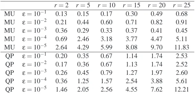
Table 1: Unconstrained NMF. Comparison between QP algorithm and multiplicative updates (MU). A medium-sized computer vision data set, V _∈R1200×150, was factorized using multiplicative updates and the QP algorithm (Alg. 3.1) using different numbers of basis functions r and different accuraciesε. Average run time in seconds over 10 repeated runs is reported. Overall, the QP algorithm shows similar performance to multiplicative up-dates.

6. Experiments

In this section we perform comparisons with established algorithms on artificial and on real-world data sets to validate our results from a practical point of view. We also provide evidence that the local sparsity maximization seems not prone to end in bad local optima. Finally, we show that the supervised constraints from eqn. (7) can lead to NMF codes that are more useful for recognition.

6.1 Unconstrained NMF

In a first experiment, we validated that the quadratic programming algorithm (Tab. 3.1) yields results similar to the fast and stable multiplicative update (MU) algorithm by Lee and Seung (2000). To this end, we factorized a data set from facial expression classification (Buciu and Pitas, 2004; Lyons et al., 1998) using both algorithms on subproblems of different sizes and different requirements for accuracy. To make a fair comparison, we ensured that the reconstruction error f(W,H) =_kV₋ W H_kF of the QP algorithm was at least as small as the corresponding error from a previous run

of the MU algorithm. We performed 10 repeated runs, each time starting from a randomly chosen initialization W,H that was identical for both methods. The results2 are summarized in Tab. 1. Both methods perform well on the data set. MU has an edge with the smaller problems, while QP has advantages when high accuracies are required. Overall, both methods are practical for solving real-world problems.

0 20 40 0

50 100

0 10 20 0

0.5 1

0 20 40 0

50

0 10 20 0

0.5 1

0 20 40 0

100 200

0 10 20 0

0.5 1

0 20 40 0

50

0 10 20 0

0.5 1

(a) Ground truth W and H.

5 10 15 20

5 10 15 20 25 30 35 40

(b) X=W H+η.

0 10 20 30 40 0

20 40

0 5 10 15 20 0

1 2

0 10 20 30 40 0

20 40

0 5 10 15 20 −5

0 5

0 10 20 30 40 0

2 4

0 5 10 15 20 0

2 4

0 10 20 30 40 0

2 4

0 5 10 15 20 0

2 4

(c) Recovered bases using smin_w =0.0.

0 10 20 30 40 0

50

0 5 10 15 20 0

1 2

0 10 20 30 40 0

20 40

0 5 10 15 20 0

2 4

0 10 20 30 40 0

20 40

0 5 10 15 20 0

1 2

0 10 20 30 40 0

5 10

0 5 10 15 20 −5

0 5

(d) Recovered bases using smin_w =0.6.

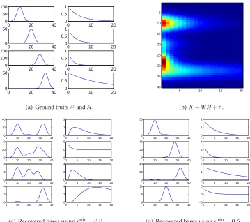
Figure 2: Paatero experiments. The entries of the factors W and H are displayed (Figure 2(a)) as well as the resulting data matrix X (Figure 2(b)). In the experiments, a small amount of Gaussian noiseη_∼

N

6.2 Sparsity-Controlled NMF

To examine the performance of the sparsity-controlled NMF algorithms we repeated an experiment suggested by Paatero (1997). Here, a synthetic data set consisting of products of Gaussian and exponential distributions is analyzed using NMF. This data set (Figure 2(a)) is designed to resemble data from spectroscopic experiments in chemistry and physics and is not easily analyzed: without prior knowledge, NMF is reported to fail to recover the original factors in the data set. As a remedy, Paatero hints that a “target shape” extension to NMF is beneficial. We will show that for this data set imposing an additional min-sparsity constraint on W is sufficient to lead to correct factorizations.

smin_w 0.0 0.2 0.4 0.6 0.8

TPC # correct results 0 0 0 7 4

TPC med run time (sec.) 20.7 16.8 14.5 53.7 117.2

TPC min obj. value 0.26 0.26 0.24 0.25 210.57

SMA # correct results 0 0 0 9 0

SMA med run time (sec.) 142.0 113.3 60.3 54.1 14.0

SMA min obj. value 0.25 0.26 0.24 0.26 161.5

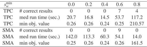
Table 2: Sparsity-controlled NMF. Statistics of the Paatero experiment collected over 10 runs for the tangent-plane constraints (TPC) and the sparsity-maximization algorithm (SMA). The number of correct reconstructions (see text), the median run time, and the best objective value obtained are reported for different choices of the sparsity constraint. Correct recon-structions are found in seven resp. nine out of ten trials for a sufficiently strong sparsity constraint: smin_w =0.6. This quota can be increased at the expense of longer running times.

consistent with Paatero (1997), the basis functions are not recovered correctly without additional prior information in the form of constraints. Also, the objective value f(W,H) =_kV₋W H_kF

is not indicative of correct results. Only for the extremely sparse case with smin_w =0.8 did we obtain noticeably worse objective values. However, not shown in the table, for the interesting case

smin_w =0.6 the objective values of the correct recoveries were all below 0.4 while from the remaining incorrect recoveries each was above 5.0. Thus, while the objective value is not useful for model selection purposes it seems to indicate good solutions once a suitable model is defined.

Finally, we point out that for the correct value of the sparsity constraint the number of correct recoveries is essentially a function of the stopping parameters. With more conservative stopping parameters one can ensure that in every single case bases are recovered correctly. But then running times increase. In our experiment we favored a short run time over perfect success rate. Accordingly, the best combination of W and H was found after just 9 seconds of computation.

6.3 Global Approaches

A potential source of difficulties with the sparsity-maximization algorithm is that the lower bound on sparsity is optimized only locally in (38). Through the proximity constraint in (40) the amount of sparsity obtained in effect limits the step size of the algorithm. Insufficient sparsity optimization may, in the worst case, lead to convergence to a bad local optimum.

To see if this worst-case scenario is relevant in practice, we discretized the problem by sampling the sparsity cones using rotated and scaled version of the current estimate Hk and then evaluated

f(W,H)using samples from each individual sparsity cone. Then we picked one sample from each cone and computed (38) replacing the starting point Hkby the sampled coordinates. For an exhaus-tive search on r cones each sampled with s points we have srstarting points to consider.

For demonstration we used the artificial data set from Paatero (1997) consisting of products of Gaussian and exponential functions (Figure 2). This data set is suitable since it is not overly large and sparsity control is crucial for its successful factorization.

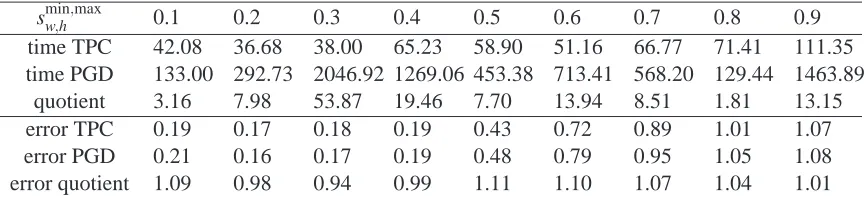
smin_w,h,max 0.1 0.2 0.3 0.4 0.5 0.6 0.7 0.8 0.9

time TPC 42.08 36.68 38.00 65.23 58.90 51.16 66.77 71.41 111.35

time PGD 133.00 292.73 2046.92 1269.06 453.38 713.41 568.20 129.44 1463.89

quotient 3.16 7.98 53.87 19.46 7.70 13.94 8.51 1.81 13.15

error TPC 0.19 0.17 0.18 0.19 0.43 0.72 0.89 1.01 1.07

error PGD 0.21 0.16 0.17 0.19 0.48 0.79 0.95 1.05 1.08

error quotient 1.09 0.98 0.94 0.99 1.11 1.10 1.07 1.04 1.01

Table 3: Comparison. Tangent-plane constraint (TPC) algorithm and projected gradient descent (PGD). The algorithms were used to find sparse decompositions of the CBCL face data set. TPC outperforms PGD w.r.t. computational effort (measured in seconds) while keeping errors small.

then combined the samples on each cone in each possible way and evaluated g for all corresponding starting points. In a second experiment we placed 1000 points on each sparsity cone, and randomly selected 104 combinations as starting points. The best results obtained over four runs and 80 iter-ations with our local linearization method used in SMA and the sparse enumeration (first) and the sampling (second) strategy, are reported below:

Algorithm min-sparsity objective value

SMA 0.60 0.24

sparse enumeration 0.60 0.26

sampling 0.60 0.26

We see that the local sparsity maximization in SMA yields results comparable to the sampling strategies. In fact, it is better: Over four repeated runs the sampling strategies each produced outliers with very bad objective values (not shown). This is most likely caused by severe under-sampling of the sparsity cones. This problem is not straightforward to circumvent: With above sampling schemes a run over 80 iterations takes about 24h of computation, so more sampling is not an option. In comparison, the proposed algorithm finishes in few seconds.

6.4 Real-World Data and Comparison with PGD

For a test with real-world data we used the CBCL face data set (CBCL, 2000). For different values of the sparsity constraints we derived NMF bases (Figure 1) and examined reconstruction error g and training time. In this experiment we used the tangent-plane constraints method and smin_w =smax_w =

smin_h =smax_h . For comparison, we also employed the projected gradient descent (PGD) algorithm from Hoyer (2004) using the code provided on the author’s homepage3. While the comparison in speed should be taken with a grain of salt—both methods use very different stopping criteria—the results (Tab. 3) show that the TPC method is competitive in speed and quality of its solutions.

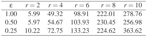
6.5 Large-Scale Factorization of Image Data

To examine performance on a larger data set we sampled 10 000 image patches of size 11_×11 from the Caltech-101 image database (Fei-Fei et al., 2004). Using a QP solver (Remark 5) and the TPC

ε r=2 r=4 r=6 r=8 r=10

1.00 5.99 49.32 98.91 222.01 278.76

0.50 5.97 54.67 103.93 230.45 256.98

0.25 10.22 72.75 133.23 224.62 363.62

Table 4: Large-scale performance. A matrix containing n =10 000 image patches with m= 121 pixels was factorized using r basis functions and different stopping criteria for the TPC/QP algorithm (see text). The median CPU time (sec.) for three repeated runs is shown. Even the largest experiment with over 100 000 unknown variables is solved within 6 min.

algorithm we computed image bases with r=2,4, . . . ,10 and r=50 basis functions using smin_w =0.5. In addition, we varied the stopping criterion fromε_{∈ {}1,0.5,0.25_}. Note that the corresponding QP instances contained roughly 100 000 to over half a million unknowns, so a stopping criterion ofε=1 translates to very small changes in the entries of W and H. We did not use any batch processing scheme but solved the QP instances directly, requiring between 100 MB and 2 GB of memory.

We show the median CPU time over three repeated runs for this experiment in Table 4: While the stopping criterion has only minor influence on the run time the number of basis functions is critical. All problems with up to 10 basis functions are solved within 6 min. For the large problem with 50 basis functions we measured a CPU time of 3, 5, and 7 hours forε_{∈ {}1,0.5,0.25_}. Mem-ory consumption was roughly 2 GB. We conclude that factorization problems with half a million unknowns can be comfortably solved on current office equipment.

6.6 Supervised NMF

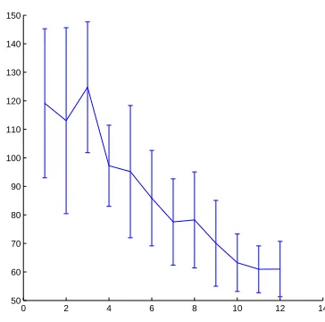
We examined how supervised NMF contributes to solve a classification task. Using overall 100 training samples we trained an r=4 dimensional NMF basis for the digits 0, 3, 5, and 8 from the opt-digits database. Subsequently, the remaining 1421 opt-digits were classified using the nearest neighbor classifier. The penalty parameterλin (7) was chosen asλ= (∞,5,2,1,0.75,0.5,0.4,0.3,0.2,0.1,

0.05,0.01), where∞corresponds to classical NMF without class label information. The experiment was repeated 30 times, and the mean classification error is depicted in Figure 3. For comparison, a nearest-neighbor classification using a PCA basis of equal dimension generated 109 errors on the test data. It is evident that by strengthening the supervised label constraint we reduce the classifica-tion error significantly, increasing recogniclassifica-tion accuracy by a factor of two.

7. Conclusion

We have shown that Euclidean NMF with and without sparsity constraints fits nicely within the framework of sequential quadratic and second order cone programming. For these problems, progress in numerical analysis has lead to highly efficient solvers which we exploit.

avail-0 2 4 6 8 10 12 14 50

60 70 80 90 100 110 120 130 140 150

# errors

Figure 3: Supervised NMF. Reduction of classification error by supervised NMF. The letters 8, 5, 3, and 0 from the optdigits database are classified using a NMF basis of dimension

m=4 and overall 100 training and 1421 test samples. From left to right various values for the supervised label constraint,λ= (∞,5,2,1,0.75,0.5,0.4,0.3,0.2,0.1,0.05,0.01), were applied. Each experiment was repeated 30 times, mean performance and standard deviations of the nearest neighbor classificator are reported. Asλdecreases the super-vised label constraint is strengthened, reducing the classification error by a factor of two.

able in supervised classification settings leads to additional convex constraints that do not further complicate the optimization problem in a noteworthy way: no new algorithms need to be derived, no suitable, typically more stringent, learning rates need to be determined.

Acknowledgments

The authors thank P. O. Hoyer for making his NMF-pack software publicly available. We also thank Bo Jensen for answering any question about the MOSEK solver quickly and reliably. Last but not least we thank the anonymous reviewers for their valuable comments.

References

D. P. Bertsekas. Nonlinear Programming. Athena Scientific, Belmont, Massachusetts, 1999.

I. Buciu and I. Pitas. Application of non-negative and local non negative matrix factorization to facial expression recognition. In Proc. of Intl. Conf. Pattern Recogn. (ICPR), pages 288–291, 2004.

A. Chichocki, R. Zdunek, and S. Amari. Csisz´ar’s divergences for non-negative matrix factorization: Family of new algorithms. In 6th Intl. Conf. on ICA and Blind Sign. Separ., March 2006.

D. Donoho and V. Stodden. When does non-negative matrix factorization give a correct decompo-sition into parts? In Adv. in Neur. Inform. Proc. Syst. (NIPS), volume 17, 2004.

L. Fei-Fei, R. Fergus, and P. Perona. Learning generative visual models from few training examples: an incremental Bayesian approach tested on 101 object categories. In Comp. Vis. and Pattern

Recogn. (CVPR) 2004, Workshop on Generative-Model Based Vision, 2004.

C. A. Floudas and V. Visweswaran. A primal-relaxed dual global optimization approach. J. of

Optim. Theory and Applic., 78(2), 1993.

A. Graham. Kronecker Products and Matrix Calculus With Applications. Ellis Horwood Lim., Chichester, 1981.

M. Heiler and C. Schn¨orr. Reverse-convex programming for sparse image codes. In Proc. of Energy

Minim. Methods in Comp. Vision and Pattern Recog. (EMMCVPR), volume 3757 of LNCS, pages

600–616. Springer, 2005.

J. B. Hiriart-Urruty. Generalized differentiability, duality and optimization for problems dealing with differences of convex functions. In J. Ponstein, editor, Lect. Not. Econom. Math. Systems, volume 256, pages 37–70. Springer, 1985.

R. Horst and H. Tuy. Global Optimization. Springer, Berlin, 1996.

P. O. Hoyer. Non-negative sparse coding. Proc. of the IEEE Works. on Neur. Netw. for Sig. Proc., pages 557–565, 2002.

P. O. Hoyer. Non-negative matrix factorization with sparseness constraints. J. of Mach.

Learn-ing Res., 5:1457–1469, 2004.

P. O. Hoyer and A. Hyv¨arinen. A multi-layer sparse coding network learns contour coding from natural images. Vision Research, 42(12):1593–1605, 2002.

Cplex 2001. ILOG CPLEX 7.5 User’s Manual. ILOG Inc., France, 2001.

D. D. Lee and H. S. Seung. Algorithms for non-negative matrix factorization. In Adv. in Neur.

Inform. Proc. Syst. (NIPS), 2000.

D. D. Lee and H. S. Seung. Learning the parts of objects by non-negative matrix factorization.

Nature, 401(21):788–791, October 1999.

S. Z. Li, X. W. Hou, H. J. Zhang, and Q. S. Cheng. Learning spatially localized, parts-based representation. In Proc. of Comp. Vision and Pattern Recog. (CVPR), 2001.

M. S. Lobo, L. Vandenberghe, S. Boyd, and H. Lebret. Applications of second-order cone program-ming. Linear Algebra and its Applications, 284:193–228, 1998.

H. D. Mittelmann. An independent benchmarking of SDP and SOCP solvers. Math. Programming,

Series B, 95(2):407–430, 2003.

Mosek 2005. The MOSEK optimization tools version 3.2 (Revision 8) User’s manual and reference. MOSEK ApS, Denmark, 2005.

P. Paatero. Least squares formulation of robust non-negative factor analysis. Chemometrics and

Intelligent Laboratory Systems, 37, 1997.

P. Paatero and U. Tapper. Positive matrix factorization: A non-negative factor model with optimal utilization of error estimates of data values. Environmetrics, 5:111–126, 1994.

R. T. Rockafellar and R. J.-B. Wets. Variational Analysis, volume 317 of Grundlehren der math. Wissenschaften. Springer, 1998.

J. Shen and G. W. Isra¨el. A receptor model using a specific non-negative transformation technique for ambient aerosol. Atmospheric Environment, 23(10):2289–2298, 1989.

I. Singer. Minimization of continuous convex functionals on complements of convex subsets of locally convex spaces. Math. Oper. Statist. Ser. Optim., 11:221–234, 1980.

P. Smaragdis and J. C. Brown. Non-negative matrix factorization for polyphonic music transcription. In IEEE Workshop on Appl. of Sign. Proc. to Audio and Acoustics, pages 177–180, 2003.

J. F. Sturm. Using SeDuMi 1.02, a Matlab toolbox for optimization over symmetric cones (updated

version 1.05). Department of Econometrics, Tilburg University, Tilburg, The Netherlands, 2001.

J. F. Toland. A duality principle for nonconvex optimization and the calculus of variation.

Arch. Rat. Mech. Anal., 71:41–61, 1979.

H. Tuy. D.c. optimization: Theory, methods and algorithms. In R. Horst and M. Pardalos, editors,

Handbook of global optimization, pages 149–216. Kluwer, Dordrecht-Boston-London, 1995.

H. Tuy. Convex programs with an additional reverse convex constraint. J. of Optim. Theory and

Applic., 52(3):463–486, March 1987.

Y. Wang, Y. Jia, C. Hu, and M. Turk. Fisher non-negative matrix factorization for learning local features. In Proc. Asian Conf. on Comp. Vision, 2004.

S. J. Wright. Primal–Dual Interior–Point Methods. SIAM, 1996.

W. Xu, X. Liu, and Y. Gong. Document clustering based on non-negative matrix factoriza-tion. In SIGIR ’03: Proc. of the 26th Ann. Intl. ACM SIGIR Conf. on Res. and

Devel-opm. in Info. Retrieval, pages 267–273. ACM Press, 2003. ISBN 1-58113-646-3. doi:

http://doi.acm.org/10.1145/860435.860485.