Multiplicative Multitask Feature Learning
Xin Wang [email protected]
Department of Computer Science and Engineering University of Connecticut
Storrs, CT 06279, USA
Jinbo Bi [email protected]
Department of Computer Science and Engineering University of Connecticut
Storrs, CT 06279, USA
Shipeng Yu [email protected]
Health Services Innovation Center Siemens Healthcare
Malvern, PA 19355, USA
Jiangwen Sun [email protected]
Department of Computer Science and Engineering University of Connecticut
Storrs, CT 06279, USA
Minghu Song [email protected]
Worldwide Research and Development Pfizer Inc.
Groton, CT 06340, USA
Editor:Urun Dogan, Marius Kloft, Francesco Orabona, and Tatiana Tommasi
Abstract
formulations by comparing with the state of the art, which provides instructive insights into the feature learning problem with multiple tasks.
Keywords: Multitask learning, regularization, sparse modeling, blockwise coordinate descent
1. Introduction
Multitask learning (MTL) improves the generalization of the estimated models for multi-ple related learning tasks by capturing and exploiting the task relationships. It has been theoretically and empirically shown to be more effective than learning tasks individually. Especially when single task learning suffers from limited sample size, multitask learning re-inforces a single learning process with the transferable knowledge learned from the related tasks. Multi-task learning has been widely applied in many scientific fields, such as robotics (Zhang and Yeung, 2010), natural language processing (Ando and Zhang, 2005), computer aided diagnosis (Bi et al., 2008), and computer vision (Kang et al., 2011).
Research efforts have been devoted to various MultiTask Feature Learning (MTFL) algo-rithms. One direction of these works directly learns the dependencies among tasks, either by modeling the correlated regression or classification noise (Greene, 2002), or assuming that the model parameters share a common prior (Yu et al., 2005; Lee et al., 2007; Xue et al., 2007; Yu et al., 2007; Jacob et al., 2008), or by examining the tasks’ covariance matrix (Bonilla et al., 2007; Zhang and Yeung, 2010; Guo et al., 2011; Yang et al., 2013). Another research direction relies on a basic assumption that the different tasks may share a sub-structure in the feature space. In order to exploit this shared subsub-structure, Rai and Daume (2010) project the task parameters to explore the latent common substructure. Kang et al. (2011) form a shared low-dimensional representation of data by feature learning. More recent methods explore the latent basis that can be used to characterize the entire set of tasks and examine the potential clusters of tasks. For instance, Passos et al. (2012) assume that subsets of features may be shared only between tasks in the same cluster. Kumar and Daume III (2012) allow overlapping of tasks in different groups by having several bases in common. Maurer et al. (2013) exploit a dictionary allowing sparse representations of the tasks. Gong et al. (2012) detect if certain tasks are outliers from the majority of the tasks. Regularization methods are widely used in MTFL to learn a shared subset of features. A common strategy is to impose a blockwise joint regularization (Meier et al., 2008; Zhao et al., 2009) on all task model parameters to shrink the effects of features across the tasks and simultaneously minimize the regression or classification loss. These methods employ the so-called `1,p matrix norm (Lee et al., 2010; Liu et al., 2009a; Obozinski and Taskar,
2006; Zhang et al., 2010; Zhou et al., 2010) that is the sum of the `p norms of the rows in
a matrix. As a result, this regularizer encourages sparsity among the rows. If a row of the parameter matrix corresponds to a feature and a column represents an individual task, the
`1,pregularizer intends to rule out the unrelated features across tasks by shrinking the entire
rows of the matrix to zero. Typical choices forpare 2 (Obozinski and Taskar, 2006; Evgeniou and Pontil, 2004) and∞ (Turlach et al., 2005). Effective algorithms have since then been developed for the `1,2 (Liu et al., 2009a) and `1,∞ (Quattoni et al., 2009) regularization.
Later, the`1,p norm is generalized to include 1< p≤ ∞with a probabilistic interpretation
normal prior for all tasks (Zhang et al., 2010). Although the matrix-norm based regularizers lead to convex learning formulations for MTFL, recent studies show that a convex regularizer may be too relaxed to approximate the `0-type regularizer for the shrinkage effects in the
feature space and thus results in suboptimal performance (Gong et al., 2013). To address this problem, non-convex regularizers, such as the capped-`1, `1 regularizer (Gong et al.,
2013), have been proposed for the multitask joint regularization. However, using non-convex regularizers may bring up computational challenges. For instance, non-convex formulations are usually difficult to solve, and require more complicated optimization algorithms to guarantee satisfactory performance.
For the existing MTFL methods based on joint regularization, a major limitation is that it either selects a feature as relevant to all tasks or excludes it from all models, which is very restrictive in practice where tasks may share some features but may also have their own specific features that are not relevant to other tasks. To overcome this limitation, one of the most effective strategies is to decompose the model parameters into either summation (Jalali et al., 2010; Chen et al., 2011; Gong et al., 2012) or multiplication (Xiong et al., 2006; Bi et al., 2008; Lozano and Swirszcz, 2012) of two components with separate regularizers applied to the two components. One regularizer is imposed on the component taking care of the task-specific model parameters and the other one is imposed on the component for mining the cross-feature sparsity. Specifically, for the methods that decompose the parameter matrix into summation of two matrices, the dirty model in (Jalali et al., 2010) employs `1,1 and `1,∞ regularizers to the two components. A robust MTFL method in
(Chen et al., 2011) uses the trace norm on one component for mining a low-rank structure shared by tasks and a column-wise `1,2-norm on the other component for identifying task
outliers. A more recent method applies the`1,2-norm both row-wisely to one component and
column-wisely to the other (Gong et al., 2012). For these additive decomposition methods, it requires the corresponding entries in both components to be zero in order to exclude a feature from a task.
For the methods that work with multiplicative decompositions, the parameter vector of each task is decomposed into an element-wise product of two vectors where one is used across tasks and the other is task-specific. To exclude a feature from a task, the multi-plicative decomposition only requires one of the components to be zero. Existing methods of this line apply the same regularization to both of the component vectors, by either the
`2-norm penalty (Bi et al., 2008), or the sparse `1-norm (i.e., multi-level LASSO (Lozano
• We propose and examine a general framework of the multiplicative decomposition that enables a variety of regularizers to be applied. The general form corresponds to a family of MTFL methods, including all early methods that decompose model parameters as a product of two components (Bi et al., 2008; Lozano and Swirszcz, 2012).
• Our theoretical analysis has revealed that this family of methods is actually equiv-alent to the joint regularization based approach but with a more general form of regularizers, including matrix-norm based and non-matrix-norm based regularizers. The non-matrix-norm based joint regularizers derived from the proposed framework have never been considered previously. If they are considered in the joint regulariza-tion form, the resultant optimizaregulariza-tion problems will be difficult to solve. However, our equivalent multiplicative MTFL framework in this case uses convex regularizers on the two components, which can be solved efficiently.
• Further analysis reveals that the optimal solution of the across-task component can be analytically computed by a formula of the optimal task-specific parameters. This ana-lytical result facilitates a better understanding of the shrinkage effects of the different regularizers applied to the two components.
• Statistical justification is also derived for this family of formulations. It proves that the proposed framework is equivalent to maximizing a lower bound of themaximum a posteriorsolution under a probabilistic model that assumes generalized normal priors on model parameters.
• Two new MTFL formulations are derived from the proposed general framework. Un-like the existing methods (Bi et al., 2008; Lozano and Swirszcz, 2012) where the same kind of vector norm is applied to both components, the shrinkage of the global and task-specific parameters differs in the new formulations. We empirically illustrate the scenarios where the two new formulations are more suitable for solving the MTFL problems.
• An efficient blockwise coordinate descent algorithm is derived suitable for solving the entire family of the methods. Given some of the methods (including the two new formulations we study) correspond to non-matrix-norm based joint regularizers, our algorithm provides a powerful alternative to solving the related difficult optimization problems, allowing us to explore the behaviors and properties of these regularizers in an effective way. Convergence analysis is thoroughly discussed.
Table 1: The regularization terms used in various MTFL methods.
Model Methods Norms
Joint reg-ularization models
A
Evgeniou and Pontil (2004) `1,2
Turlach et al. (2005) `1,∞ Lee et al. (2010) both`1,1and`1,2
Zhang et al. (2010) `1,p,1< p≤ ∞ Gong et al. (2012) capped`1,1
Decomposed models
A=P+Q Jalali et al. (2010) `1,1 onP,`1,∞ onQ Gong et al. (2012) `1,2onP,`1,2onQT
A= diag(c)·B
The proposed framework (`k)k onc, (`p)p onB
Bi et al. (2008) k=2, p=2
Lozano and Swirszcz (2012) k=1, p=1
The new formulation 1 k=1, p=2
The new formulation 2 k=2, p=1
The rest of the paper is organized as follows. Section 2 defines the mathematical nota-tion and introduces the proposed models in detail. Secnota-tion 3 discusses several important theoretical properties of the proposed models including equivalence analysis. Section 4 provides the statistical justification of the multiplicative MTFL models. In Section 5, we develop an efficient algorithm to solve the optimization problems in the proposed models with a convergence analysis. Section 6 shows the empirical results, in which simulations have been designed to examine the various feature sharing patterns for which a specific choice of regularizer may be preferred. Extensive experiments with a variety of classifica-tion and regression benchmark data sets are also described in Secclassifica-tion 6. In Secclassifica-tion 7, we conclude this work.
2. The Proposed Multiplicative MTFL
GivenT tasks in total, for each taskt,t∈ {1,· · ·, T}, we have sample set (Xt∈R`t×d,yt∈ R`t). The data set ofXthas`texamples, where thei-th row corresponds to thei-th example
xti of task t, i ∈ {1,· · ·, `t}, and each column represents a feature and there are totally d
features. The vector yt contains yt
i, the label of the i-th example of task t. We consider
functions of the linear form yt = α>t xti where αt ∈ Rd, which corresponds to computing
Xtαton the training data as the estimate of yt. We define the parameter matrix or weight
matrixA= [α1,· · ·,αT] and denote the rows ofA byαj,j ∈ {1,· · ·, d}.
The joint regularization based MTFL method with the `1,p regularizer minimizes T
X
t=1
L(αt,Xt,yt) +λ
d
X
j=1
||αj||p, (1)
for the best αt:t=1,···,T, where L(αt,Xt,yt) is the loss function of task t which computes
the discrepancy between the observed yt and the model output Xtαt, and λ is a tuning
parameter to balance between the loss and the regularizer. Although any suitable loss function can be used in the formulation (1), convex loss functions are the common choices such as the least squares lossP`t
i=1(yit−α >
P`t
i=1log(1 +e−y
t
i(α>txti)) for classification problems. These loss functions are strictly convex
with respect to the model parameters αt. The `p norm is computed for each row of the
matrix A corresponding to a feature (rather than a task) so to enforce sparsity on the features.
A family of multiplicative MTFL methods can be derived by rewriting αt= diag(c)βt
where diag(c) is a diagonal matrix with its diagonal elements composing a vectorc. The c
vector is used across all tasks, indicating if a feature is useful for any of the tasks, and the vector βt is only for task t. Let j index the entries in these vectors. We have αtj = cjβjt.
Typically c comprises binary entries that are equal to 0 or 1, but the integer constraint is often relaxed to require just non-negativity (c≥0). We minimize a regularized loss function as follows for the bestc and βt:t=1,···,T:
min
βt,c≥0 T
P
t=1
L(c,βt,Xt,yt) +γ1
T
P
t=1
||βt||pp+γ2||c||kk, (2)
whereL(c,βt,Xt,yt) is the same loss function used in Eq.(1) but with αt replaced by the
new vector of (cjβjt)j=1,···,d, ||βt|| p
p = Pdj=1|βjt|p and ||c||kk = Pdj=1(cj)k, which are the
`p-norm of βt to the power of p and the `k-norm of c to the power of k if p and k are
positive integers. The tuning parameters γ1,γ2 are used to balance the empirical loss and
regularizers. At optimality, if cj = 0, the j-th variable is removed for all tasks, and the
corresponding row vectorαj =0; otherwise the j-th variable is selected for use in at least
one of the α’s. Then, a specific βt can rule out thej-th variable from taskt ifβjt= 0. If bothp=k= 2, Problem (2) becomes the formulation used in Bi et al. (2008). Since the`2-norm regularization is applied on bothβtand c, this model does not impose strong
sparsity on the model parameters. According to our empirical study, this model may be suitable for the scenarios where only a few features can be excluded from all of the tasks, and the different models (tasks) share a lot features between each other. There could exist features that, although irrelevant to most of the tasks, cannot be completely excluded only due to few tasks.
If p = k = 1, Problem (2) becomes the formulation used in Lozano and Swirszcz (2012), where the `1-norm regularization is applied on βt and c and thus it induces very
strong sparsity both on task-specific parameters and the across-task component to select the features. Compared to the model in Bi et al. (2008), this model is more suitable for learning from the tasks with persistently sparse models. For example, many features are irrelevant to any of the tasks, and only a few of the features selected by c are used by an individual task, indicating the sparse pattern in sharing the selected features among tasks. Besides the above two existing models, any other choices of p and k will derive into new formulations for MTFL. Note that the two existing methods discussed in Bi et al. (2008); Lozano and Swirszcz (2012) use p=k in their formulations, which rendersβjt and
cj the same amount of shrinkage. To explore other feature sharing patterns among tasks,
we propose two new formulations wherep6=k.
Formulation 1:
Ifp= 2 but k= 1 in Problem (2), then we obtain the following optimization problem
min
βt,c≥0 T
P
t=1
L(c,βt,Xt,yt) +γ1
T
P
t=1
||βt||2
When there exists a large subset of features irrelevant to any of the tasks, it requires a sparsity-inducing norm on c. However, within the relevant features selected by c, the majority of these features are shared between tasks. In other words, the features used in each task are not sparse relative to the features selected byc, which requires a non-sparsity-inducing norm onβ. Hence, we use`1 norm oncand`2 norm on eachβin our formulation
(2).
Formulation 2:
Ifp= 1 but k= 2 in Problem (2), we obtain the following optimization problem
min
βt,c≥0 T
P
t=1
L(c,βt,Xt,yt) +γ1
T
P
t=1
||βt||1+γ2||c||22. (4)
When the union of the features relevant to any given tasks includes many or even all features, the`2 norm penalty oncmay be preferred. However, only a limited number of features are
shared between tasks, i.e., the features used by individual tasks are sparse with respect to the features selected as useful across tasks by c. We can impose the`1 norm penalty onβ.
Clearly, many other choices of p and kvalues can be used, such as those corresponding to higher order polynomials (e.g.,Pd
j=1c3j). Our theoretical results in the next few sections
apply to all positive value choices of p and k unless otherwise specified. In our empirical studies, however, we have implemented algorithms for the two existing models and the two new models for comparison. Some other choices of regularizers may require significant re-programming of our algorithms and we will leave them for more thorough individual examinations in the future.
3. Theoretical Analysis
We first extend the formulation (1) to allow more choices of regularizers. We introduce a new notation that is an operator applied to a vector, such as αj. The operator ||αj||p/qp =
q
q PT
t=1|αtj|p, p, q ≥ 0, which corresponds to the `p norm if p = q and both are positive
integers. A joint regularized MTFL approach can solve the following optimization problem with pre-specified values of p,q and λ, for the best parametersαt:t=1,···,T:
min
αt T
P
t=1
L(αt,Xt,yt) +λ
d
P
j=1
q
||αj||p/q
p . (5)
Our main results of this paper include (i) a theorem that establishes the equivalence between the models derived from solving Problem (2) and Problem (5) for properly chosen values of
λ,q,k,γ1 and γ2; (ii) a theorem that delineates the conditions for (2) to impose a convex
(or concave) regularizer on the model parameter matrix A; and (iii) an analytical solution of Problem (2) forc which shows how the sparsity of the across-task component is relative to the sparsity of task-specific components.
Theorem 1 (Main Result 1) Let αˆt be the optimal solution to Problem (5) and (βˆt, ˆc)
be the optimal solution to Problem (2). Then αˆt =diag(ˆc) ˆβt when λ= 2
q
γ2−
p kq
1 γ
p kq
2 and
Proof Theorem 1 can be proved by establishing the following two lemmas and two the-orems. The two lemmas provide the basis for the proofs of the two theorems and then from the first theorem, we conclude that the solution ˆαt of Problem (5) also minimizes the
following optimization problem:
min
αt,σ≥0
PT
t=1L(αt,Xt,yt) +µ1Pdj=1σ −1 j ||αj||
p/q
p +µ2Pdj=1σj, (6)
and the optimal solution of Problem (6) also minimizes Problem (5) when proper values of λ, µ1 and µ2 are chosen. The second theorem connects Problem (6) to the proposed
formulation (2). We show that the optimal ˆσj is equal to (ˆcj)k, and then the optimal ˆαcan
be computed as diag(ˆc) ˆβt from the optimal ˆβt.
Note that whenp= 2 andq= 1, the intermediate problem (6) uses a similar regularizer to that in Micchelli et al. (2013) where |ασj|2
j +σj is used to approximate|α
j|in the` 1-norm
regularizer. Problem (6) extends the discussion in Micchelli et al. (2013) to include more general regularizers according to pand q.
Lemma 2 For any givenαt:t=1,···,T, Problem (6) can be optimized with respect to σ by the
following analytical solution
σj =µ
1 2
1µ −1
2
2
q
||αj||p/q
p . (7)
Proof By the Cauchy-Schwarz inequality, we can derive a lower bound for the sum of the
two regularizers in Problem (6) as follows:
µ1
d
X
j=1
σj−1||αj||p/qp +µ2 d
X
j=1
σj ≥2
√
µ1µ2
d
X
j=1
q
||αj||p/q
p , (8)
where the equality holds if and only ifσj =µ
1 2
1µ −12 2
q
||αj||p/q
p .
Using the method of proof by contradiction, suppose that σ∗ optimizes Problem (6)
with a given set of αt:t=1,···,T, but σ∗j 6= µ
1 2
1µ −1
2
2
q
||αj||p/q
p . Thus, σ∗ does not make
the regularization term reach its lower bound. Then, we can choose another ˜σ where
˜
σj =µ
1 2
1µ −1
2
2
q
||αj||p/q
p , so ˜σ delivers the lower bound in Eq.(8). Because the lower bound
(the right hand side of Eq.(8)) only depends on α, it is a constant for fixed αt:t=1,···,T.
Hence, since the loss function is also fixed for given αt:t=1,···,T, ˜σ reaches a lower objective
value of Problem (6) than that ofσ∗, which contradicts to the optimality ofσ∗. Therefore, the optimalσ always takes the form of Eq.(7).
Remark 3 Based on the proof of Lemma 2, we also know that the objective function of (5)
is the lower bound of the objective function of (6) for any given αt (including the optimal
ˆ
αt) whenλ= 2
√
µ1µ2, and the lower bound can be attained if and only ifσ is set according to the formula (7). Hence, we can also conclude that if ( ˆαt,σˆ) is the optimal solution of
Problem (6), then σˆj =µ
1 2
1µ −1
2
2
q
Lemma 4 Let αtj = cjβjt for all t and j. Replacing βt by αt in Problem (2) yields the following optimization problem
min
αt,c≥0 T
P
t=1
L(αt,Xt,yt) +γ1Pdj=1c
−p j ||αj||
p
p+γ2Pdj=1(cj)k. (9) For any given αt:t=1,···,T, Problem (9) can be optimized with respect to c by the following analytical solution
cj = (γ1γ2−1
T
X
t=1
(αtj)p)p+1k. (10)
Proof This lemma can be proved following a similar argument in the proof of Lemma
2. By the Cauchy-Schwarz inequality, the sum of the two regularizers in (9) satisfies the following inequality
γ1
d
X
j=1
c−jp||αj||pp+γ2 d
X
j=1
ckj ≥2γ
k p+k
1 γ
p p+k
2 d
X
j=1
(||αj||pp)p+kk, (11)
and the equality holds if and only if γ1c−jp||αj|| p
p =γ2ckj (and note that all parameters γ1,
γ2,||αˆj||pp and c are non-negative), which yields the following formula
cj = (γ1γ2−1
T
X
t=1
(αtj)p)p+1k.
Through proof by contradiction, we know that the optimalchas to take the above formula.
Based on Lemma 2, we will prove that Problem (5) is equivalent to Problem (6) in the sense that an optimal solution of Problem (5) is also an optimal solution of Problem (6) and vice versa when λ,µ1, and µ2 satisfy certain conditions.
Theorem 5 The solution sets of Problem (5) and Problem (6) are identical when λ =
2√µ1µ2.
Proof First, if ˆA = [ ˆαt:t=1,···,T] minimizes Problem (5), we show that the pair ( ˆA,σˆ)
minimizes Problem (6) where ˆσj =µ
1 2
1µ −1
2
2
q
||αˆj||p/qp .
By Remark 3, the objective function of (5) is the lower bound of the objective function
of (6) for any given A (including the optimal solution ˆA). When ˆσj =µ
1 2
1µ −12 2
q
||αˆj||p/qp ,
Problem (6) reaches the lower bound. In this case, Problem (5) at ˆA and Problem (6) at ( ˆA,σˆ) have the same objective value. Now, suppose that the pair ( ˆA,σˆ) does not minimize Problem (6), there exists another pair ( ˜A,σ˜)6= ( ˆA,σˆ) that achieves a lower objective value
than that of ( ˆA,σˆ). By Lemma 2, we have that ˜σj =µ
1 2
1µ −1
2
2
q
||α˜j||p/qp , and then Problem
when λ= 2√µ1µ2. In other words, the objective values of (6) and (5) are identical at ˜A.
Hence, ˜Aachieves a lower objective value than that of ˆAfor Problem (5), contradicting to the optimality of ˆA.
Second, if ( ˆA,σˆ) minimizes Problem (6), we show that ˆA minimizes Problem (5). Suppose that ˆA does not minimize Problem (5), which means that there exists ˜αj
(6= ˆαj for some j) that achieves a lower objective value than that of ˆαj. We set ˜σj =
µ 1 2
1µ −12 2
q
||α˜j||p/qp . Then ( ˜A,σ˜) is an optimal solution of Problem (6) as proved in the first
paragraph, and will bring the objective function of Problem (6) to a lower value than that of ( ˆA,σˆ), contradicting to the optimality of ( ˆA,σˆ).
Therefore, Problems (5) and (6) have identical solution sets when λ= 2√µ1µ2.
In order to link Problem (6) to our formulation (2), we letσj = (cj)k,k∈R,k6= 0 and
αjt =cjβjt for all tand j, and derive an equivalent objective function of Problem (6) based
on Lemmas 2 and 4.
Theorem 6 The optimal solution ( ˆA,σˆ) of Problem (6) is equivalent to the optimal
so-lution ( ˆB,ˆc) of Problem (2) where αˆtj = ˆcjβˆtj and σˆj = (ˆcj)k when γ1 = µ
kq 2kq−p
1 µ
kq−p 2kq−p
2 ,
γ2 =µ2, and k= 2qp−1.
Proof First, if ˆαtj and ˆσj optimize Problem (6), we show that ˆcj = k
p
ˆ
σj and ˆβjt = ˆαtj/cˆj
optimize Problem (2).
By a change of variables (replacing ˆαt and ˆσ by ˆβt and ˆc in Problem (6)), we know
that ˆβt and ˆc minimize the following objective function
J( ˆβtj,cˆj) = T
X
t=1
L(ˆc,βˆt,Xt,yt) +µ1 d
X
j=1
||βˆj||p/qp cˆj(p−kq)/q+µ2
d
X
j=1
(ˆcj)k. (12)
By Lemma 2 and Remark 3, the optimal ˆσj = µ
1 2
1µ −1
2
2
q
||αˆj||p/qp . Because ˆcj = k
p
ˆ
σj, we
derive that
ˆ
cj =
µ1µ−12 ||βˆ j
||p/qp
q 2kq−p
.
Substituting the formula of ˆcj into Eq.(12) yields the same objective function of Problem
(2) after replacing µ1 and µ2 by γ1 and γ2 with the equationsγ1 =µ
kq 2kq−p
1 µ
kq−p 2kq−p
2 , γ2 =µ2.
Therefore, ˆβt and ˆc optimize Problem (2) because otherwise, if any other solution (β,c) can further reduce the objective value of Problem (2), then the correspondingαand σ will bring the objective function of Problem (6) to a lower value than ˆα and ˆσ.
Next, if ˆβjtand ˆcj optimize Problem (2), we show that ˆαtj = ˆcjβˆtjand ˆσj = (ˆcj)koptimize
Problem (6).
Substituting ˆαtj, ˆσj for ˆβjt, ˆcj in Problem (2) yields an objective function
J( ˆαtj,σˆj) = T
X
t=1
L( ˆαt,Xt,yt) +γ1 d
X
j=1
||αˆj||ppσˆ−(j p/k)+γ2
d
X
j=1
ˆ
We hence know that ˆαtj and ˆσj minimize Eq.(13). Similar to the proof of Lemma 4, we can
show that the optimal ˆσ takes the form of
ˆ
σj = (γ1γ−12 )
k
k+p(||αˆj||p p)
k k+p.
Substituting the formula into Eq.(13) and setting γ1 =µ
kq 2kq−p
1 µ
kq−p 2kq−p
2 and γ2 =µ2 transfer
Eq.(13) to the objective function of Problem (6). Thus, ˆαtj and ˆσj optimize Problem (6).
Now, based on the above two lemmas and two theorems, we can derive that when
λ= 2
q
γ2−
p kq
1 γ
p kq
2 andq = k+p
2k , the optimal solutions to Problems (2) and (5) are equivalent.
Solving Problem (2) will yield an optimal solution ˆα to Problem (5) and vice versa. By the equivalence analysis, the proposed framework corresponds to a family of joint regularization methods as defined by Eq.(5). Assuming a convex loss function is used, this family includes some convex formulations when convex regularizers are applied to A in (5) and some other non-convex formulations when non-matrix-norm based regularizers are applied to A. Particularly, when q = p/2, the regularization term on αj in (5) becomes the standard `p-norm. Correspondingly, when k = p/(p−1) which is commonly not an
integer except p = 2, our formulation (2) amounts to imposing a `1,p-norm on A. When
both k and p take positive integers (exceptp=k= 2), Problem (2) is equivalent to using a non-matrix-norm regularizer in (5). Combinations of differentp and k values will render the models different algorithmic behaviors.
Theorem 7 (Main Result 2)For any positivekandp, ifkp≥k+p, then the formulation
(2) imposes a convex regularizer on the model parameter matrixA; or otherwise, it imposes a concave regularizer onA.
Proof According to Theorem 1, the formulation (2) is equivalent to the formulation (5)
that imposes the following regularizer onA:
λ
d
X
j=1
q
||αj||p/q
p =λ d
X
j=1
(||αj||p) p 2q =λ
d
X
j=1
(||αj||p) kp
k+q. (14)
whereq = k2+kp and λ= 2
q
γ2−
p kq
1 γ
p kq
2 .
A functionxa is a convex function in terms ofx >0 ifa≥1; or otherwise, it is concave. Hence, if kp ≥ k+p, Eq.(14) is a composite function of two functions: a convex function
xkkp+p and another convex function which is the `
p vector norm of αj. Thus, the overall
regularizer is convex. Otherwise, if kp < k+p, the regularizer becomes a concave function in terms ofα’s.
Remark 8 For a particular choice of p= 2 and k= 2, Problem (2) is formulated as
min
βt,c≥0 T
P
t=1
L(c,βt,Xt,yt) +γ1
T
P
t=1
||βt||2
which is used in Bi et al. (2008). This problem is equivalent to the following joint regular-ization method as used in Obozinski and Taskar (2006); Argyriou et al. (2007).
min
αt T
X
t=1
L(αt,Xt,yt) +λ
d
X
j=1
v u u t
T
X
t=1
(αt
j)2, (16)
when λ= 2√γ1γ2. Problem (16) uses the so called `1,2-norm to regularize the matrix A.
Remark 9 For a particular choice of p= 1 and k= 1, Problem (2) is formulated as
min
βt,c≥0 T
P
t=1
L(c,βt,Xt,yt) +γ1
T
P
t=1
||βt||1+γ2||c||1, (17)
which is used in Lozano and Swirszcz (2012). This problem is equivalent to the following joint regularization method
min
αt T
X
t=1
L(αt,Xt,yt) +λ
d
X
j=1
v u u t
T
X
t=1
|αt
j|, (18)
whenλ= 2√γ1γ2. Problem (17) imposes stronger sparsity onβ andc(and correspondingly onα) than (15), which intends to shrink more model parameters to zero. Problem (18) uses a concave non-matrix-norm regularizer.
Remark 10 For a particular choice of p = 2 and k = 1, which corresponds to the new
formulation (3). This problem is equivalent to the following joint regularization method
min
αt T
X
t=1
L(αt,Xt,yt) +λ
d
X
j=1
3
v u u t
T
X
t=1
(αtj)2, (19)
whenλ= 2γ 1 3
1γ
2 3
2. Problem (19) uses a concave non-matrix-norm regularizer as well but the concavity is weaker than Problem (18) in the sense that the polynomial order is 23 rather than 12.
The proposed formulation (3) imposes stronger sparsity induction on the across-task component than on the task-specific component. Thus, it has stronger shrinkage effects to exclude many features for all the tasks. If the jth feature is considered as unrelated to most of the tasks, the model of p = k = 2 may shrink cj to a small value but not zero,
the new model (3) might shrink cj to zero instead. Therefore this model would be more
Remark 11 For a particular choice of p = 1 and k = 2, which corresponds to the new formulation (4). This problem is equivalent to the following joint regularization method
min
αt T
X
t=1
L(αt,Xt,yt) +λ
d
X
j=1
3
v u u t
T
X
t=1
|αt
j|
!2
, (20)
whenλ= 2γ 2 3
1γ
1 3
2. Problem (20) uses another concave non-matrix-norm regularizer that has the similar polynomial order of 23 to Problem (19). In comparison with (19), the cross-task quadratic terms (e.g.,|α1
j||α2j|,|α2j||α3j|) are allowed inside the cube root in this formulation.
The new formulation (4) imposes stronger sparsity induction on task-specific component than on the across-task vector. This model can be favorable in the cases where few tasks share a limited number of selected features. As shown in our empirical results, for instance, when every two or three tasks share a limited subset of selected features but no common features are used by more than three tasks, this model performs the best among the four multiplicative MTFL formulations. In comparison to the model in Lozano and Swirszcz (2012), this model allows more of the features that are only relevant to a few tasks to be selected. In comparison with the model in Bi et al. (2008), this model can help to remove a lot of irrelevant or redundant features for individual tasks from the selected features.
We further derive another main result that characterizes the optimal across-task vector as a formula of the optimal task-specific vectors. This connection can be easily developed from the above equivalence analysis, and can help us understand the relationship and in-teraction between the two components.
Theorem 12 (Main Result 3) Let βˆt,t= 1,· · · , T,be the optimal solutions of Problem
(2), Let Bˆ = [ ˆβ1,· · · ,βˆT] and βˆj denote the j-th row of the matrixBˆ. Then,
ˆ
cj = (γ1/γ2)
1 k k
v u u t
T
X
t=1
( ˆβjt)p, (21)
for all j= 1,· · ·, d, is optimal to Problem (2).
Proof This analytical formula can be directly derived from Theorem 5 and Theorem
6. When we set ˆσj = (ˆcj)k and ˆαjt = ˆcjβˆjt in the proof of Theorem 6, we obtain ˆcj =
µ1µ−12 ||βˆ j
||p/qp
q
2kq−p
. In the same proof, we also show thatµ1=γ
2kq−p kq
1 γ
p−kq kq
2 andµ2 =γ2.
Substituting these formulas into the formula of c yields ˆcj = (γ1/γ2)
1 k||βˆj||
p
2kq−p.
More-over, to establish the equivalence between (2) and (5), we require q = k2+kp, which leads to
k= 2kq−p. Hence,||βˆj||2kqp−p = k
q PT
t=1( ˆβjt)p. We then obtain the formula (21).
Remark 13 For particular choices of p and k, the relation between the optimal c and β
Table 2: The shrinkage effect of c with respect toβ for four common choices ofp and k.
p k c
2 2 cˆj =
q
γ1γ2−1
q PT
t=1( ˆβjt)2
1 1 cˆj =γ1γ2−1
PT t=1|βˆjt|
2 1 cˆj =γ1γ2−1
PT
t=1( ˆβjt)2
1 2 cˆj =
q
γ1γ2−1
q PT
t=1|βˆjt|
4. Probabilistic Interpretation
In this section we show that the proposed multiplicative formalism is related to themaximum a posteriori(MAP) solution of a probabilistic model. Letp(A|∆) be the prior distribution of the weight matrix A = [α1, . . . ,αT] = [α1>, . . . ,αd>]> ∈ Rd×T, where ∆ denote the
parameter of the prior. Then thea posterioridistribution ofAcan be calculated via Bayes rule as
p(A|X,y,∆)∝p(A|∆)
T
Y
t=1
p(yt|Xt,αt). (22)
Denote z ∼ GN(µ, ρ, p) the univariate generalized normal distribution, with the density function
p(z) = 1
2ρΓ(1 + 1/p)exp
−|z−µ|
p
ρp
, (23)
in which ρ >0, p >0, and Γ(·) is the Gamma function (Goodman and Kotz, 1973). Now let each element of A,αt
j, follow a generalized normal prior, αtj ∼ GN(0, δj, p). Then with
theindependent and identically distributed assumption, the prior takes the form (also refer to Zhang et al. (2010) for a similar treatment)
p(A|∆)∝
d
Y
j=1 T
Y
t=1
1
δj
exp−|α
t j|p
δjp
=
d
Y
j=1
1
δT
j
exp−kα
jkp p
δpj
, (24)
where k · kp denotes the vector p-norm. With an appropriately chosen likelihood function
p(yt|Xt,αt) ∝ exp(−L(αt,Xt,yt)), finding the MAP solution is equivalent to solving the
following problem:
min A,∆ J =
T
X
t=1
L(αt,Xt,yt) +
d
X
j=1
kαjkpp
δpj +Tlnδj
. (25)
Setting the derivative ofJ with respect to δj to zero, we obtain:
δj =
p
T
1/p
Bringing this back to (25), we have the following equivalent problem:
min
A J =
XT
t=1L(αt,Xt,yt) +T
Xd
j=1lnkα jk
p. (27)
Now let us look at the multiplicative nature ofαtj with different p∈[1,∞). When p= 1, we have:
d
X
j=1
lnkαjk1= d X j=1 ln T X t=1
|αtj|
! = d X j=1 ln T X t=1
|cjβjt|
!
=
d
X
j=1
ln|cj|+ ln T
X
t=1
|βjt|
!
≤
d
X
j=1
|cj|+
d X j=1 T X t=1
|βjt| −2d,
where the inequality is because of the fact that lnz ≤ z−1 for any z >0. Therefore we can optimize an upper bound ofJ in (27),
min A J1 =
T
X
t=1
L(αt,Xt,yt) +T
d
X
j=1
|cj|+T
d X j=1 T X t=1
|βjt| −2dT, (28)
which is equivalent to the multiplicative formulation (2) where{p, k}={1,1}. This proves the following theorem:
Theorem 14 When {p, k}={1,1}, optimizing the multiplicative formulation (2)is
equiv-alent to maximizing a lower bound of the MAP solution under probabilistic model (22)with
p= 1 in the prior definition.
In the general case, we have:
d
X
j=1
lnkαjkp =
1 p d X j=1 ln T X t=1
|cjβjt|p
! = 1 p d X j=1
ln (ckj)pk · T
X
t=1
|βjt|p
! = 1 k d X j=1
ln|cj|k+1
p d X j=1 ln T X t=1 |βt
j|p
≤ 1
k
d
X
j=1
|cj|k+1
p
T
X
t=1
kβtkp
p−d(
1
k+
1
These inequalities lead to an upper bound of J in (27). By minimizing the upper bound, the problem is formulated as:
min
A Jp,k=
T
X
t=1
L(αt,Xt,yt) +
T
kkck
k k+
T p
T
X
t=1
kβtkpp, (29)
which is equivalent to the general multiplicative formulation in (2). Therefore we have proved the following theorem:
Theorem 15 Optimizing the multiplicative formulation (2), in the form of (29), is
equiv-alent to maximizing a lower bound of the MAP solution under probabilistic model (22)with
p∈(1,∞) in the prior definition.
5. Optimization Algorithm
Alternating optimization algorithms have been used in both of the early methods (Bi et al., 2008; Lozano and Swirszcz, 2012) to solve Problem (2) which alternate between solving two subproblems: solve forβtwith fixedc; solve forc with fixedβt. The convergence property of such an alternating algorithm has been analyzed in Bi et al. (2008); Lozano and Swirszcz (2012) that it converges to a local minimizer. In these early methods, both of the two subproblems have to be solved using iterative algorithms such as gradient descent, linear or quadratic program solvers.
Besides the algorithm that solves for c and βt alternatively and can be applied to our formulations, we design an alternating optimization algorithm that utilizes the closed-form solution forcwe have derived in Lemma 4 and the property that both Problems (2) and (5) are equivalent to the intermediate Problem (6) (or Problem (9)). In the algorithm to solve Problem (2), we start from an initial choice ofc. At iterations, we start fromcs, and solve
forβst with the fixed cs. We then compute the value ofαst = diag(cs)βst, which is used to updatecs tocs+1 according to Eq.(10) in Lemma 4. The overall procedure is summarized
inAlgorithm 1. As a central idea in designing this algorithm, at each iteration we update
βto reduce the loss function, and updatec to reduce the regularizer while maintaining the same loss function value. Note that if the value ofαis fixed, the loss will remain the same.
To analyze the convergence property of Algorithm 1, we utilize the fact that Problem (2) and Problem (9) are equivalent. For notational convenience, we denote the objective function of Problem (2) by g(B,c) that takes inputs βt and c. We denote the objective function of Problem (9) by f(A,c). Both objective functions comprise the sum of three parts. For instance, f can be written as follows:
f(A,c) =f0(A,c) +fA(A) +fc(c), (31)
wheref0(A,c) =γ1Pdj=1(c −p j
PT
t=1(αtj)p) is the part that involves bothα andc,fA(A) =
P
tL(αt,Xt,yt) is the part relying only on α, andfc(c) = µ2Pdj=1(cj)k is the part for c
only. Letzbe the vector consisting of all variables in Problem (9). Similar to what has been defined in Tseng (2001), we define that the pointz is a stationary point of f ifz∈dom f
wheredom f is the feasible region off, and
lim
Algorithm 1 The blockwise coordinate descent algorithm for multiplicative MTFL
Input: Xt,yt,t= 1,· · ·, T, as well asγ1,γ2,p and k
Initialize: cj = 1,∀j= 1,· · ·, d, and s= 1
repeat
Compute ˜Xt=Xtdiag(cs),∀ t= 1,· · · , T
fort= 1,· · · , T do
Solve the following problem for βst
min
βt
L(βt,X˜t,yt) +γ1||βt||pp (30)
end for
Compute αst = diag(cs)βst
Sets=s+ 1
Compute cs+1 using αst according to Eq.(10)
until maxt,j(|(αtj)s−(αtj)s−1|)< (or other proper termination rules)
Output: αt,c andβt,t= 1,· · · , T
where b denotes any feasible direction, (which corresponds to 5f(z) = 0 if f is differen-tiable, or0 ∈∂f(z) iff is non-differentiable where∂f(z) is the subgradient off atz). In our case,f is not differentiable atα= 0 orc= 0 whenp is set to an odd number. We also define that a pointzis a coordinate-wise minimum point off ifz∈dom f, and∀bk ∈Rdk
that makes (0,· · · ,bk,· · · ,0) a feasible direction, there exists a small >0, such that for
all positiveλ≤,
f(z+λ(0,· · · ,bk,· · · ,0))≥f(z), (33)
wherek indexes the blocks of variables in our algorithm, which include α1,· · · ,αT and c,
so k ={1,· · ·, T + 1}, and the (T + 1)-th block is for c, dk is the number of variables in
thekth coordinate block and in our casedk =d. The vector (0,· · · ,bk,· · ·,0) is a vector
inRd×(T+1) and used to only varyz in thek-th block.
We first prove that for the sequence of points generated by Algorithm 1, the objec-tive function f is monotonically non-increasing. Then we prove the sequence of points is bounded, because of which, the sequence will have accumulation points. We prove that each accumulation point is a coordinate-wise minimum point. Then according to Tseng (2001), iff is regular at an accumulation point z∗, this z∗ is a stationary point.
Lemma 16 Let the sequence of iterates generated by Algorithm 1 be zs = {As,cs}
s=1,2,··· and the functionf is defined by (31), thenf(As+1,cs+1)≤f(As,cs).
Proof First, note that for each {As,cs}, we accordingly have {Bs,cs} where αs
t =
∀j and t. Then, g( ˜Bs,cs+1) =f(As,cs+1). Next in Algorithm 1, we obtain Bs+1 by solv-ing Problem (30), i.e., by optimizsolv-ing g with respect B when c is fixed to cs+1. Hence,
g(Bs+1,cs+1) ≤ g( ˜Bs,cs+1). Then A will be updated by As+1 = diag(cs+1)Bs+1, which leads tof(As+1,cs+1) =g(Bs+1,cs+1). Overall, we have
f(As+1,cs+1) =g(Bs+1,cs+1)≤g( ˜Bs,cs+1) =f(As,cs+1)≤f(As,cs).
This proves thatf(As+1,cs+1)≤f(As,cs).
Based on the proof of Lemma 16, we can also show that g(Bs+1,cs+1) ≤g(Bs,cs) for the sequence of {Bs,cs}s=1,2,··· that is also created by Algorithm 1.
Lemma 17 The sequence of iterates generated by Algorithm 1, zs = {As,cs}s=1,2,···, (or
equivalently, {Bs,cs}
s=1,2,···) is bounded.
Proof According to Lemma 16, we know thatf(As+1,cs+1)≤f(As,cs), andg(Bs+1,cs+1)≤
g(Bs,cs), ∀s= 1,2,· · ·. Hence, g(Bs,cs) ≤g(B1,c1), ∀s = 1,2,· · ·. Let g(B1,c1) = C.
Then,g(Bs,cs) is upper bounded by C.
In our algorithm, we assume that the loss function ingcan be either the least squares loss or the logistic regression loss of all the tasks. Hence, the loss terms are non-negative (actually most other loss functions, such as the hinge loss, are also non-negative). The two regulariz-ers, one onβtand the other onc, are both non-negative. Thus, we have that||βst||pp ≤C/γ1
and ||cs||k
k ≤ C/γ2, ∀s = 1,2,· · ·. This shows that the sequence of {B
s,cs}
s=1,2,··· is
bounded. Becauseαst = diag(cs)βst,||αst||pp =Pdj=1|(αtj)s|p =Pdj=1|(csj(βjt)s|p ≤ ||cs||22pp+
||βst||22pp ≤ C˜ where ˜C is a constant computed from C, γ1 and γ2. Thus, the sequence of
zs ={As,cs}s=1,2,··· is also bounded.
Theorem 18 The sequencezs ={As,cs}
s=1,2,··· generated by Algorithm 1 has at least one accumulation point. For any accumulation point z∗ = {A∗,c∗}, z∗ is a coordinate-wise minimum point of f.
Proof According to Lemma 17, the sequence zs is bounded, so there exists at least one
accumulation point z∗ and a subsequence of{zs}
s=1,2,··· that converges toz∗. Without loss
of generality and for notational convenience, let us just assume that {zs}
s=1,2,··· converges
toz∗. Becausez∗is an accumulation point, if it is the iterate at the current iterations, then in the next iteration s+ 1, the same iterate z∗ will be obtained. Hence, β∗t is the optimal solution of Problem (30) whencis set toc∗ (and all otherβk6=t=β∗k). Correspondingly,c∗
is the optimal solution of Problem (2) whenBis set toB∗. Hence, for any feasible direction
(0,· · ·,bt,· · ·,0),∀t= 1,2,· · ·, T + 1, we have
f(z∗+λ(0,· · ·,bt,· · · ,0))≥f(z∗), (34)
Theorem 19 If both p and k are positive, and k ≥ 1, the accumulation point z∗ is a stationary point of f.
Proof Due to Lemma 4, we know that the optimal solution of Problem (9) can only occur
whencandαtsatisfy Eq.(10), so any other points can be excluded from discussion. Hence,
we define a new level set Z0 = {z|f(z) ≤ C} ∩ {z|cj = (γ1γ2−1
PT
t=1(αtj)p)
1 p+k,∀αt
j}. We
now prove that f is continuous on this setZ0 and the gradient of f exists when p is even (differentiable case), and examine0∈∂f atz∗ for non-differentiable cases.
Given the definition of f,f is continuous with respect toαt
j, ∀j and t. Because f0 is a
division term that has a divisor based oncj, we have thedivision-by-0 issue, sof is in general
not continuous with respect to cj at 0 (but continuous and differentiable at other values).
However, using L’Hospital’s rule (i.e., lim
φ→0 f1(φ)
f2(φ) = limφ→0
f10(φ)
f0
2(φ), we show thatf is continuous
with respect to cj at cj = 0 in the set Z0. When cj = 0, ||αj||pp =PTt=1(αtj)p = 0 due to
Eq.(10). Let φ=||αj||pp. Since the function f0 is a ratio of two items both approaching 0
as functions ofφ, we can apply L’Hospital’s rule as follows
lim
φ→0
||αj||p
p
(cj)p
= lim
φ→0
φ
(γ1γ2−1φ)
p p+k
= lim
φ→0
1
p p+k(γ1γ
−1 2 )
p p+kφ−
k p+k
= lim
φ→0
(p+k)φp+kk
p(γ1γ2−1)
p p+k
= 0.
We then compute the partial derivative off0 with respect tocj, which is ∂f∂c0j =
−p||αj||p p
(cj)p+1 for cj 6= 0. Now whencj approaches 0, we can prove continuity using L’Hospital’s rule:
∂f0
∂cj
|cj→0 = lim φ→0
−p||αj||p
p
(cj)p+1
= lim
φ→0
−pφ
(γ1γ2−1φ)
p+1 p+k
= lim
φ→0
−p(p+k)φkp−+k1
(p+ 1)(γ1γ−12 )
(p+1) p+k
= 0,
when k > 1. When k = 1, the limit is a finite number −p(p+k)/((p+ 1)(γ1γ2−1)
(p+1) p+k ).
Note that when an odd p is taken, ||αt||pp = P|αtj|p is not differentiable at 0. However,
the above limit exists no matterf is differentiable or not because we takeφas the varying parameter. With the above conditions, we use the results in Tseng (2001) that when each subproblem has a unique minimum, which is the case in our algorithm because Subproblem (30) is strictly convex (for our chosen loss functions) and we have already proved the unique analytical solution of c,z∗ is a stationary point off.
We briefly discuss the computation cost of Algorithm 1. Subproblem (30) is essentially for single task learning, which can be solved by many existing efficient algorithms, such as gradient-based optimization methods. The second subproblem has a closed-form solution for
c, which requires only a minimal level of computation. The computation cost of Algorithm 1 only linearly increases with the number of tasks. Due to the nature of Algorithm 1, it can be easily parallelizable and distributed to multiple processors when optimizing individual
6. Experiments
We empirically evaluated the performance of the multiplicative MTFL algorithms on both synthetic data sets and a variety of real-world data sets, where we solved either classifica-tion (using the logistic regression loss) or regression (using the least squares loss) problems. In the experiments, we implemented and compared Algorithm 1 for four parameter set-tings: (p, k) = (2,2), (1,1), (2,1), and (1,2), corresponding to four multiplicative MTFL (MMTFL) methods as listed in Table 2. Although when the values of (p, k) were (2,2) and (1,1), the two models corresponded respectively to the same methods in Bi et al. (2008) and Lozano and Swirszcz (2012), they were solved differently from prior methods using our Algorithm 1 with higher computational efficiency. When (p, k) = (2,1) and (1,2), the resultant models corresponded to the two new formulations.
In our experiments, the multiplicative MTFL methods were also compared with the additive MTFL methods that decompose the model parameters into an addition of two components, such as the Dirty model (DMTL) (Jalali et al., 2010) and the robust MTFL (rMTFL) (Gong et al., 2012). Single task learning (STL) approaches were also implemented as baselines and compared with all of the MTFL algorithms in the experiments. We list the various methods used for comparison in our experiments as follows:
• STL lasso : Learning each task independently with ||αt||1 as the regularizer.
• STL ridge : Learning each task independently with||αt||22 as the regularizer.
• DMTL (Jalali et al., 2010) : The dirty model with regularizers ||P||1,1 and ||Q||1,∞,
whereA=P+Q.
• rMTFL (Gong et al., 2012) : Robust multitask feature learning with the regularizers
||P||1,2 and ||QT||1,2, where A=P+Q.
• MMTFL{2,2} (Bi et al., 2008) : Multiplicative multitask feature learning with regu-larizers||B||2
F and ||c||22, where A= diag(c)B.
• MMTFL{1,1}(Lozano and Swirszcz, 2012) : Multiplicative multitask feature learning with regularizers ||B||1,1 and ||c||1, whereA= diag(c)B.
• MMTFL{2,1}(New formulation 1) : Multiplicative multitask feature learning with regularizers||B||2
F and ||c||1, where A= diag(c)B.
• MMTFL{1,2}(New formulation 2) : Multiplicative multitask feature learning with regularizers||B||1,1 and ||c||2
2, whereA= diag(c)B.
In all experiments, unless otherwise noted, the original data set was partitioned to have 25%, 33% or 50% of the data in a training set and the rest used for testing. For each specified partition ratio (corresponding to a trial), we randomly partitioned the data 15 times and reported the average performance. The same tuning process was used to tune the hyperparameters (e.g.,γ1 and γ2) of every method in the comparison. In every trial, an
2kwithk=−10,−9,· · · ,7. In the subsequent partitions of each trial, the hyperparameters were fixed to the values that yielded the best performance in the CV.
The regression performance was measured by the coefficient of determination, denoted byR2, which measures the explained variance of the data by the fitted model. In particular, we used the following formula to report performanceR2 = 1−
Pn
i=1(yi−fi)2
Pn
i=1(yi−¯y)2 where ¯y is the
mean of the observed values ofy and fi is the prediction of the observedyi. The reported
values in our experiments were the averagedR2 over all tasks. TheR2value ranges from 0 to 1, and a higher value indicates better regression performance. The classification performance was measured by the F1 score, which is the harmonic mean of precision and recall. The numbers we reported in each trial was the F1 score averaged over all tasks. Similarly, the F1 score also ranges from 0 to 1 and higher values represent better classification performance.
6.1 Simulation Studies
We created three categories of data sets, all of which were designed for regression experi-ments to evaluate the behaviors of the different methods. The data sets in each category were created with a pre-specified feature sharing structure. The first two categories were designed to validate the scenarios that we hypothesized for our two new formulations to work. We performed sensitivity analyses using these two categories of data sets, i.e., study-ing how performance was altered when the number of tasks or the number of features varied. Because we also empirically compared with a few additive decomposition based methods, it would be interesting to see how multiplicative MTFL behaved in a scenario that was actu-ally in favor of additive MTFL. Hence, in the third category, the feature sharing structure was generated following the assumption that the robust MTFL method used (Gong et al., 2012).
In all experiments, we created input examples Xt for each task t using a number of
features randomly drawn from the standard multivariate Gaussian distributionN(0,1), and pre-defined A = [α1,· · · ,αT] across all tasks. The responses for each task was computed
by yt=Xtαt+t wheret∼ N(0,0.5) was the noise introduced to the model. If an entry
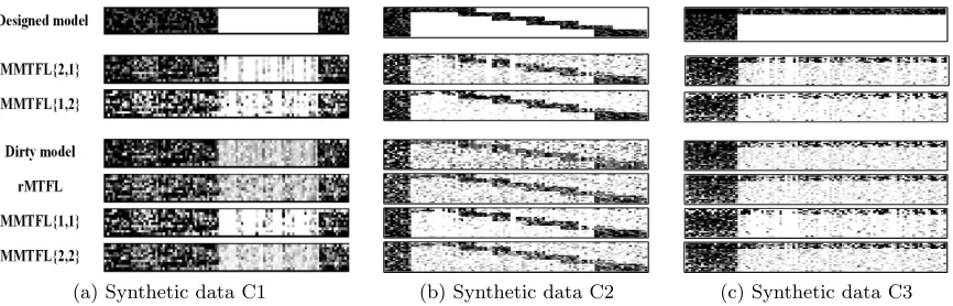
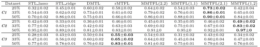
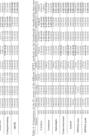
of A was set to non-zero, its value was randomly sampled from a uniform distribution in the interval [0.5,1.5]. As a side note, we transposedA in Figure 1 for better illustration.
6.1.1 Synthetic Datasets
non-matrix-norm-(a) Synthetic data C1 (b) Synthetic data C2 (c) Synthetic data C3
Figure 1: The true parameter matrix versus the parameter matrices constructed by the var-ious methods on synthetic data. The figure shows the results when 200 examples and 100 features were created for 20 tasks each. Darker color indicates larger values in magnitude.
based regularizers. We hypothesized that the proposed new formulation (3) would produce better regression performance than existing models on this data category.
To examine how the number of tasks influenced the performance of different methods, we varied the number of tasks from 1, 5, 10, 50, and 100 to 1000. For each task, we created 200 examples, each represented by 100 features. We also tested the different methods when increasing the number of features. In this set of experiments, we used 20 tasks and each task contained 1000 examples. Each example was represented by a number of features ranging from 200 to 1000 with a step size of 200.
Category 2 (C2). In the C2 experiments, 10% of the rows in A were set to non-zero and these features were shared by all tasks. We then arranged the tasks to follow six different sparse structures (the staircases) as shown in Figure 1b(top), where we once again transpose A. Each of the remaining features except the 10% common features was used by a comparatively small proportion of the tasks. Consecutive tasks were grouped such that the neighboring groups of tasks shared 7% of the features besides the 10% common features, whereas the non-neighboring groups of tasks did not share any features. Therefore, no feature could be excluded from all tasks, but a majority of individual features (90%) was only useful for few tasks (i.e., the useful features for one task were sparse). In this case, the non-sparsity-inducing norm was suitable for regularizingc and sparsity-inducing norm was more suitable for regularizingβ. We hypothesized that the new formulation (4) would produce better regression performance than the other models on this data set.
We created 20, 50, 100, 500 and 1000 tasks, respectively, to test the algorithms’ sensi-tivity to the number of tasks. The numbers of tasks were chosen to make sure enough tasks in each of the six groups. The number of tasks in each group ranged from 3 to 170. We generated 200 examples and 100 features for each task. We also created another set of C2 data sets with the number of features changing from 200 to 1000 with a step size of 200 for 20 tasks and 1000 examples for each task.
Table 3: Comparison of the test R2 values obtained by the different MTFL methods on synthetic data sets using different partition ratios for training data (where standard deviation 0 means that it is less than 0.01).
Dataset STL lasso STL ridge DMTL rMTFL MMTFL(2,2) MMTFL(1,1) MMTFL(2,1) MMTFL(1,2) 25% 0.32±0.02 0.45±0.01 0.60±0.02 0.58±0.02 0.64±0.02 0.54±0.03 0.73±0.02 0.42±0.04 C1 33% 0.54±0.03 0.62±0.02 0.73±0.01 0.61±0.02 0.79±0.02 0.76±0.01 0.86±0.01 0.65±0.03 50% 0.70±0.02 0.86±0.01 0.75±0.01 0.66±0.01 0.86±0.01 0.88±0.01 0.90±0.01 0.84±0.01 25% 0.42±0.03 0.33±0.01 0.36±0.01 0.46±0.01 0.45±0.01 0.35±0.05 0.46±0.02 0.49±0.02 C2 33% 0.77±0.02 0.63±0.01 0.42±0.02 0.63±0.03 0.69±0.02 0.75±0.01 0.67±0.03 0.83±0.02 50% 0.95±0.01 0.89±0.01 0.81±0.01 0.83±0.01 0.91±0 0.95±0 0.92±0.01 0.97±0 25% 0.28±0.03 0.43±0.03 0.50±0.04 0.55±0.03 0.54±0.03 0.31±0.02 0.43±0.02 0.34±0.02 C3 33% 0.47±0.01 0.56±0.02 0.60±0.02 0.65±0.02 0.64±0.02 0.45±0.04 0.60±0.04 0.47±0.03 50% 0.77±0.01 0.78±0.01 0.76±0.02 0.83±0.01 0.81±0.02 0.75±0.01 0.79±0.02 0.76±0.01
by 100 features, were generated for each of 20 tasks. The parameter matrix A = P+Q
where 80 rows in P and 16 columns in Q were set to 0. The component P was used to indicate the subset of relevant features across all tasks, and the component Qwas used to tell that there were outlier tasks that did not share features with other tasks. Given this simulation process, this data set would be in favor of the rMTFL model proposed in Gong et al. (2012). The designed model parameter matrix was shown in Figure 1c(top).
6.1.2 Performance on synthetic data sets
We first compared the regression performance of the different methods on the three cate-gories of data sets. Table 3 shows the averagedR2 values together with standard deviations for each method and each trial setting. The best results are shown in bold fonts. The results in Table 3 were obtained on synthetic data sets that had 20 tasks with 200 examples and 100 features for each task. We reported the test R2 obtained on each data set when 25%, 33% and 50% of the data were used in training. From Table 3, we observe that the pro-posed formulation (3)(MMTFL(2,1)) consistently outperformed other models on C1 data sets, whereas the proposed model (4)(MMTFL(1,2)) consistently outperformed onC2data sets. The results confirmed our hypotheses that the two proposed models could be more suitable for learning the type of sharing structures in C1and C2. As anticipated, rMTFL model constantly outperformed other models on theC3data set. Among the multiplicative MTFL methods, MMTFL(2,2) achieved similar performance to that of rMTFL (off only by 0.01∼0.02 for averageR2).
In order to elucidate the different shrinkage effects of the different decomposition strate-gies and regularizers, we compared the true parameter matrix with the constructed pa-rameter matrices by the six MTFL methods used in our experiments in Figure 1. From the results on the C1 and C2 data sets, we observe that only MMTFL(2,1), MMTFL(1,2) and MMTFL(1,1) produced reasonably sparse structures. The two additive decomposition methods could not yield a sufficient level of sparsity in the models. Although the unused features did receive smaller weights in general, they were not completely excluded. To eval-uate the accuracy of feature selection, we quantitatively measured the discrepancy between the estimated models and the true model by computing the mean squared error (MSE)
trace((A−Aest)>(A −Aest)) where Aest was the matrix estimated by a method. We
compared MSE values of individual mothods.
(a) OnC1data (b) OnC2data
Figure 2: The regression performance of different models on synthetic dataC1andC2when the number of tasks is varied.
sparse because the useful features received much smaller weights than needed (lighter than the true model). The smallest MSE was achieved by MMTFL(2,1) with a value of 0.1, and the second best model, MMTFL(1,1), had MSE = 0.2 whereas the rMTFL model had the largest MSE = 0.25.
On the C2 data, MMTFL(1,2) learned a model that was most comparable to the true model. Both MMTFL(1,2) and MMTFL(1,1) eliminated well the irrelevant features. How-ever, if we compared the two rows corresponding to these two models in Figure 1, we could see that MMTFL(1,1) broke the staircases in several places (e.g., towards the lower right and the up left corners) by excluding more features than necessary. Note that the feature sharing patterns (particularly in synthetic data C2) may not be revealed by the recent methods on clustered multitask learning that cluster tasks into groups (Kang et al., 2011; Jacob et al., 2008; Zhou et al., 2011) because no cluster structure is present in Figure 1b. Rather, the sharing pattern in Figure 1b is actually in between the consecutive groups of tasks. MMTFL(1,2) had the smallest MSE = 0.05, which was smaller than that of the second best model MMTFL(1,1) by 0.025. DMTL received the largest MSE = 0.19.
Figure 1c shows the results on the C3 data set. MMTFL(2,1), MMTFL(1,2), and
MMTFL(1,1) imposed excessive sparsity on the parameter matrix, which removed some
useful features. The other three models, DMTL, rMTFL and MMTFL(2,2), produced
similar parameter matrices, but rMTFL was originally designed to detect outlier tasks and thus was more favorable for this data set. The rMTFL model obtained the smallest MSE (0.03), and MMTFL(2,2) had a similar performance (MSE=0.04), which was the same as that of DMTL. On this data set, MMTFL(1,1) got the largest MSE (0.09). These results bring out an interesting observation that for the MTL scenarios that have outlier tasks but relevant tasks share the same set of features, MMTFL(2,2) (which corresponds to the very early joint regularized method using the`1,2 matrix norm) is most suitable among the
multiplicative MTFL methods.
(a) OnC1data (b) OnC2data
Figure 3: The regression performance of different models on synthetic dataC1andC2when the number of features is varied.
with 15 trials, and reported here the averageR2 values and standard deviation bars. From Figure 2, MMTFL(2,1) constantly performed the best among all methods on the C1 data sets (but not in the single task learning) whereas MMTFL(1,2) outperformed the other models on theC2data sets. We also observed that onC2data, MMTFL(1,1) obtained very similar performance to that of MMTFL(1,2) after the number of tasks reached 50. On this data category, almost all methods reached a stable level of accuracy after the number of tasks reached 50 except DMTL. DMTL continued to gain knowledge from more relevant tasks until it reached 500 tasks but it produced the lowestR2 values among all methods. Overall, the results indicate that with the fixed dimension and sample size, when the number of tasks reaches a certain level, the transferable knowledge learned from the tasks can be saturated for a specific feature sharing structure. On C1data, we observe that the performance was not always monotonically improved or non-degraded (for all methods) when more tasks were included, which may indicate that when an unnecessarily large number of tasks was used, it could add more uncertainty to the learning process.
Figure 3 compares the performance of different methods when we vary the number of features in the C1 and C2 categories. Obviously, when the problem dimension was higher, the learning problem became more difficult (especially when the number of tasks and sample size remained the same). All methods dropped their performance substantially with increasing numbers of features although MMTFL(2,1) and MMTFL(1,2) still outperformed other methods, respectively, on the C1 and C2 data sets. This figure also shows that MMTFL(1,1) performed well on the C2 data sets but much worse on the C1 data sets. DMTL produced good performance, close to that of MMTFL(2,1), on theC1 data sets.
6.2 Experiments with Benchmark Data
6.2.1 Benchmark Datasets
Sarcos (Argyriou et al., 2007): Sarcos data were collected for a robotics problem of learning the inverse dynamics of a 7 degrees-of-freedom SARCOS anthropomorphic robot arm. Each observation has 21 features corresponding to 7 joint positions and their velocities and accel-erations. We needed to map from the 21-dimensional input space to 7 joint torques, which corresponded to 7 tasks. For each task, we randomly selected 2000 cases for training and the remaining 5291 cases for test. Readers can consult with http://www.gaussianprocess.org/ gpml/data/ for more details.
CollegeDrinking (Bi et al., 2013): The college drinking data were collected in order to identify alcohol use patterns of college students and the risk factors associated with the binge drinking. The data set contained daily responses from 100 college students to a survey questionnaire measuring various daily measures, such as drinking expectation, negative affects, and level of stress, every day in a 30 day period. The goal was to predict the amount of nighttime drinks based on 51 daily measures for each student, corresponding to 100 regression tasks. Because there were only 30 records for each person, we used 66%, 75% and 80% of the records to form the training set, and the rest for test.
QSAR (Ma et al., 2015): The quantitative structure-activity relationship (QSAR) meth-ods are commonly used to predict biological activities of chemical compounds in the field of drug discovery. The data sets we used were collected from three different types of drug activities, including binding to cannabinoid receptor 1 (CB1), inhibition of dipeptidyl pepti-dase 4 (DPP4) and time dependent 3A4 inhibitions (TDI). For each activity, there were 200 molecule examples represented by 2618 features. Three regression models were constructed to simultaneously predict the targets−log(IC50)) of the CB1, DPP4 and TDI effectiveness based on the molecular features.
C.M.S.C. (Lucas et al., 2013): The Climate Model Simulation Crashes (C.M.S.C.) data set contained records of simulated crashes encountered during climate model uncertainty quantification ensembles. The data set comprised 3 tasks. There were 180 examples for each task. Each example was represented by an 18-dimensional feature vector. Each task is formed by a binary classification problem, which was to predict simulation outcomes (either fail or succeed) from the input parameter values for a climate model.
Landmine (Xue et al., 2007): The original Landmine data contained 29 data sets where sets 1-15 corresponded to the geographical regions that were highly foliated and sets 16-29 corresponded to the regions with bare earth or desert. Each data set could be used to build a binary classifier. We used the data sets 1-10 and 16-25 to form 20 tasks where each example was represented by 9 features extracted from radar images. The number of examples varied between individual tasks ranging from 445 to 690.
Alphadigits (Maurer et al., 2013): This data set was composed of binary 20×16 images of the 10 digits and capital letters. We used all the images of digits to form 10 binary classification tasks. For each digit, there were 39 images in this data set. We labeled the images of a single digit as positive examples, and randomly selected other 39 images from other digits and labeled them as negative examples. All the pixels were concatenated to form a 320-dimensional feature vector for each image.