Vol. 11, No. 4, 2019 Article ID IJIM-1112, 7 pages Research Article
An Effective Numerical Technique for Solving Second Order Linear
Two-Point Boundary Value Problems with Deviating Argument
M. Khaleghi ∗, E. Babolian †‡, S. Abbasbandy §
Received Date: 2017-08-13 Revised Date: 2018-05-18 Accepted Date: 2018-05-18
————————————————————————————————–
Abstract
Based on reproducing kernel theory, an effective numerical technique is proposed for solving second order linear two-point boundary value problems with deviating argument. In this method, reproducing kernels with Chebyshev polynomial form are used (C-RKM). The convergence and an error estimation of the method are discussed. The efficiency and the accuracy of the method is demonstrated on some numerical examples.
Keywords : Two-point boundary value problem; Second order boundary value problem; Deviating argument; Polynomial reproducing kernel; Chebyshev polynomials; Chebyshev reproducing kernel method.
—————————————————————————————————–
1
Introduction
B
owith different kinds of differential equationsundary value problems (BVPs) associated play important rolls to modelling a wide vari-ety of nature phenomena [1, 2, 3]. Differential equations with deviating argument have many applications such as study of problems in auto-matic control theory, problems of self-oscillating systems, long-term planning theory in economics, problems in rocket motion, a series of problems in biological science, and many other areas of sci-ence and technology. Many authors have been∗Department of Mathematics, Science and Research
Branch, Islamic Azad University, Tehran, Iran.
†Corresponding author. [email protected], Tel:
+98(912)1300842.
‡Department of Mathematics, Science and Research
Branch, Islamic Azad University, Tehran, Iran.
§Department of Applied Mathematics, Imam Khomeini
International University, Qazvin, 34149-16818, Iran.
studied the question of existence and uniqueness of a solution for this type of differential equations, see e.g. [4, 5] and references cited therein. Fi-nite differences method [4], collocation methods [10, 15], Richardson extrapolation [6], shooting techniques [7, 11], projection method [16], suc-cessive and Pad approximations [5, 12] and suc-cessive interpolations [8] are some of the existing numerical methods for boundary value problems of differential equations with deviating argument. In this paper, based on reproducing kernel with polynomial form [13, 14], we propose an effec-tive numerical technique for solving the following second order two-point boundary value problems with a deviating argument:
x′′(t) +p(t)x(t) +q(t)x(ϕ(t)) =f(t), 0≤t≤T,
x(0) =α, x(T) =β,
(1.1)
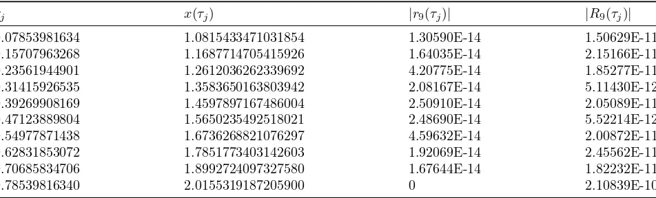
Table 1: Numerical results for Example4.1
τj x(τj) |r9(τj)| |R9(τj)|
0.07853981634 1.0815433471031854 1.30590E-14 1.50629E-11
0.15707963268 1.1687714705415926 1.64035E-14 2.15166E-11
0.23561944901 1.2612036262339692 4.20775E-14 1.85277E-11
0.31415926535 1.3583650163803942 2.08167E-14 5.11430E-12
0.39269908169 1.4597897167486004 2.50910E-14 2.05089E-11
0.47123889804 1.5650235492518021 2.48690E-14 5.52214E-12
0.54977871438 1.6736268821076297 4.59632E-14 2.00872E-11
0.62831853072 1.7851773403142603 1.92069E-14 2.45562E-11
0.70685834706 1.8992724097327580 1.67644E-14 1.82232E-11
0.78539816340 2.0155319187205900 0 2.10839E-10
whereT >0, α, β ∈R, andϕ: [0, T]→Ris such that 0≤ϕ(t)≤T,∀t∈[0, T].We suppose thatϕ is Lipschitzian, p, q ∈ C2(0, a) and f ∈ L2w[0, T] are sufficiently regular given functions such that Eq. (1.1) satisfies the existence and uniqueness of the solution. Without loss of generality, we can assume that the boundary conditions in Eq. (1.1) are homogeneous. In this paper, based on re-producing kernel theory, rere-producing kernels with polynomial form will be constructed and a com-putational method is described in order to obtain the accurate numerical solution with polynomial form of the Eq. (1.1) in the reproducing kernel spaces spanned by the Chebyshev basis polyno-mials.
2
Construction of reproducing
kernels with Chebyshev
poly-nomials
ForT >0, denote by Pn[0, T] the set of all
poly-nomials on [0, T] with real coefficients and degree less than or equal to n, namely,
Pn[0, T] :=span{1, t, t2, ..., tn} (2.2)
equipped with the following inner product
⟨x, y⟩Pn =
T ∫
0
ω(t)x(t)y(t)dt,
∀x, y∈Pn[0, T],
(2.3)
and the norm
||x||Pn=
√
⟨x, x⟩Pn, ∀x∈Pn[0, T], (2.4)
where ω is a positive weight function.
For T > 0 and positive weight function ω(t) =
T
2√T t−t2, the sequence of shifted Chebyshev
poly-nomials of the first kind in tare defined on [0, T] and can be determined as follows:
Ti∗(t) = 2(2T−1t−1)Ti∗−1(t)−Ti∗−2(t),
i≥2,
(2.5) withT0∗(t) = 1, T1∗(t) = 2T−1t−1.
The orthogonality condition is
⟨Ti∗, Tj∗⟩=
T ∫
0
ω(t)Ti∗(t)Tj∗(t)dt
=
0, i̸=j,
T π
2 , i=j= 0, T π
4 , i=j̸= 0.
(2.6)
Theorem 2.1 [13, 14] Pn[0, T] is a reproducing
kernel space and its reproducing kernel is
Rn(t, s) = n ∑
i=0
ei(t)ei(s), (2.7)
where ei(t) = { 2
T πTi∗(t), i= 0, 4
T πTi∗(t), i̸= 0.
Note that the functions in space Pn[0, T] do not
satisfy the boundary conditions of Eq. (1.1). So we define a closed subspace ofPn[0, T] by
impos-ing required homogeneous boundary conditions on it.
Definition 2.1 Let
Pn0[0, T] ={x|x∈Pn[0, T], x(0) =x(T) = 0}.
Lemma 2.1 [9] For 2 ≤ i ≤ n, the functions defined by
φi(t) = {
Ti∗(t)−1, i is even,
Ti∗(t)−2T−1t+ 1, i is odd,
(2.9)
have the property
φi(0) =φi(T) = 0, (2.10)
and for the function space Pn0[0, T], the basis functions defined by Eq. (2.9) are complete.
The orthonormal basis {φ¯i}ni=2 of Pn0[0, T] can
be deduced from Gram-Schmidt orthogonaliza-tion process using {φi}ni=2. In [13] the following closed form of ¯φi fori= 2,3, . . . , n is obtained,
¯
φi(t) =κi
Ti∗(t)−αiUi∗(t), i even,
Ti∗(t)−αiVi∗(t), i odd,
(2.11)
where κi = 2 √
(i−1)
π(i+1)T, αi = 2
i−1, Ui∗(t) =
i−2 2
∑
k=1
T2∗k(t)−12 andVi∗(t) =
i−1 2
∑
k=1
T2∗k−1(t).
Similar to the proof of Theorem 2.1, we can prove that the function space Pn0[0, T] is a reproducing kernel space and its reproducing kernel is,
Kn(t, s) = n ∑
i=2 ¯
φi(t) ¯φi(s). (2.12)
3
C-RKM for Eq. (1.1)
Let Eq. (1.1) can be transformed into the fol-lowing operator form:
{
Lx(t) =f(t), 0≤t≤T,
x(0) =x(T) = 0, (3.13)
where
Lx(t) =x′′(t) +p(t)x(t) +q(t)x(ϕ(t)), (3.14)
is a linear operator. We shall give the approx-imate solution of Eq. (3.13) in space Pn0[0, T] based on reproducing kernel theory. Let {ti}ni=0−2 be (n−1)-distinct nodes in interval [0, T]. put ψi(t) = LsKn(t, s)|s=ti, (i = 0,1, . . . , n− 2),
where the subscript s in the operator L indi-cates that the operator L applies to the func-tion s. {ψi}in=0−2 is a basis for Pn0[0, T] [13,
14]. Gram-Schmidt orthogonalization of{ψi}ni=0−2
yields{ψ¯i}ni=0−2 which is an orthonormal basis for
Pn0[0, T],
¯ ψi =
i ∑
k=0
βikψk, (βii>0, i= 0,1, . . . , n−2).
(3.15) So,xnas an approximation solution of Eq. (3.13)
in spacePn0[0, T] can be represented the following form:
xn(t) = n−2 ∑
i=0
⟨x,ψ¯i⟩Pnψ¯i(t), (3.16)
where xis the exact solution.
Theorem 3.1 If xn is the approximation
solu-tion of Eq. (3.13) in Pn0[0, T]then it can be rep-resented the following form:
xn(t) = n−2 ∑
i=0 i ∑
k=0
βikf(tk) ¯ψi(t). (3.17)
According to Eqs. (3.15) and (3.16), one obtains
⟨x,ψ¯i⟩Pn =
i ∑
k=0
βik⟨x(.),LsKn(., s)|s=tk⟩Pn
=
i ∑
k=0
βikLs⟨x(.), Kn(., s)⟩Pn|s=tk.
(3.18) Based on reproducing kernel theory and the fact that xis the exact solution, we have
⟨x,ψ¯i⟩Pn=
i ∑
k=0
βikLsx(s)|s=tk=
i ∑
k=0
βikf(tk).
(3.19) Hence,
xn(t) = n∑−2
i=0
⟨x,ψ¯i⟩Pnψ¯i(t)
=
n∑−2
i=0 i ∑ k=0
βikf(tk) ¯ψi(t).
(3.20)
To analyze the convergence and the error esti-mation in L02[0, T] = {x | x ∈ L2w[0, T], u(0) = u(T) = 0}, we define the error and the residual functions as
Rn(t) =f(t)−Lxn(t) =Lrn(t), (3.22)
where t ∈ [0, T], x ∈ L02[0, T] be the exact so-lution of Eq. (1.1) andxn is given by Eq. (3.17).
Theorem 3.2 Let x ∈ L02[0, T] be the exact
so-lution of Eq. (1.1), xn ∈ Pn0[0, T] in Eq. (3.17) be the approximation of x and for t ∈ [0, T],
rn(t) =x(t)−xn(t) then
||rn||oL2
w−→0, n−→ ∞.
From Lemma2.1and Eq. (2.11), it follows that
x(t) = ∞ ∑
i=2 ⟨
x,φ¯i ⟩
oL2 w
¯
φi(t), (3.23)
and for any integer n,i= 0,1, . . . , n−2,
⟨
¯ φi, ψi
⟩
oL2 w
= 0, j=n+ 1, n+ 2, . . . . (3.24)
Let
L02[0, T] =Pn0[0, T]⊕Pn0⊥[0, T], (3.25)
wherePn0⊥[0, T] =Span{φ¯i}∞i=n+1. So
rn ∈Pn0⊥[0, T], (3.26)
and we have
||rn||2oL2 w =||
∞ ∑
i=n+1 ⟨
rn,φ¯i ⟩
oL2 w
¯ φi||2oL2
w
= ∞ ∑
i=n+1 (
⟨
rn,φ¯i ⟩
oL2 w
)2.
Thus
||rn||oL2
w−→0, n−→ ∞. (3.27)
Theorem 3.3 For n ≥ 2 and T > 0, Let t0 <
t1 < · · · < tn−2 be any (n−1)-distinct nodes in (0, T) such that lim
n→∞t0 = 0, nlim→∞tn−2 = T. If p, q, ϕ and f ∈ Cn−1[0, T] then there exists a positive constant c such that
||rn||L2 w≤c
√
T π 2 ℏ
n−1
n , (3.28)
where ℏn= max
0≤i≤n−3{|ti+1−ti|}.
At the first, we prove that
Rn(tj) = 0, j = 0,1, . . . , n−2. (3.29)
We rewrite Eq. (3.17) as
xn(t) = n−2 ∑
i=0
Aiψ¯i(t), (3.30)
where Ai = ∑i
k=0βikf(tk). By the following
re-producing property of Kn(t, s), we have
(Lxn)(tk) = n−2 ∑
i=0
AiLtψ¯i(t)|t=tk
=
n−2 ∑
i=0
AiLt ⟨
¯
ψi(s), Kn(t, s) ⟩
|t=tk
=
n−2 ∑
i=0
Ai ⟨
¯
ψi(s),LtKn(t, s) ⟩
|t=tk
=
n−2 ∑
i=0
Ai ⟨
¯
ψi(s),LtKn(t, s)|t=tk
⟩
=
n−2 ∑
i=0
Ai ⟨
¯
ψi(s), ψk(s) ⟩
(3.31)
Note here that
j ∑
k=0
βjk(Lxn)(tk) = n−2 ∑
i=0
Ai ⟨
¯ ψi,
j ∑
k=0
βjkψk ⟩
=
n−2 ∑
i=0
Ai ⟨
¯ ψi,ψ¯j
⟩
=Aj.
(3.32)
In the above equation, putting j = 0. So, we have (Lxn(t0)) = f(t0). Similarly, taking j = 1,2, . . . , n−2 in Eq. (3.32), we obtain
(Lxn)(tj) =f(tj), j= 1, . . . , n−2. (3.33)
From the proof of theorem (3.6) in [13], there exists a positive constant dsuch that
||Rn||∞= max
t∈[0,T]|Rn(t)|≤dℏ n−1
n . (3.34)
According to the Eq. (2.6), we have
||Rn||L2 w=
√∫ T
0
ω(t)|Rn(t)|2dt≤d √
T π 2 ℏ
n−1 n .
Nothing that
rn=L−1Rn, (3.36)
then there exists a constantc such that
||rn||L2 w=||L
−1R n||L2
w≤ ||L
−1|| L2
w.||Rn||L2w
(3.37)
≤c
√
T π 2 ℏ
n−1 n .
4
Numerical examples
Example 4.1 [8] Consider the following
bound-ary value problem for t∈[0,π4],
{
x′′(t) + 2 cos(t2).x(2t) = 1 + 2(1 + t82) cos(2t), x(0) = 1, x(π4) = 1 +
√ 2 2 +
π2 32.
(4.38)
Here T = π4, ϕ(t) = λt with λ = 12. The exact solution isx(t) = t22+ sin(t) + 1, t∈[0,π4]. Apply C-RKM withn= 9, ti= π8(cos((i+1)n π) + 1), i=
0,1, . . . , n−2. Forτj = πj40, j= 1,2, . . . ,10, the
results are in Table 1, where the absolute errors |rn(τj)|and the absolute residual values|Rn(τj)|
reveal the accuracy of the method in the third and forth columns, respectively. The absolute error function|rn(t)|and the absolute residual function
|Rn(t)|are shown in Figure 1.
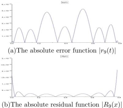
(a)The absolute error function|r9(t)|
(b)The absolute residual function|R9(x)|
Figure 1: The absolute error and residual func-tions of Example4.1
Example 4.2 For the following boundary value
problem
x′′(t)−et.x(t) +x(sin(t)) =f(t),
t∈[0,1],
x(0) = 0, x(1) = 0.
(4.39)
the exact solution isx(t) =et−et2, wheref(t) = et−e2t+et+t2 +esin(t)−esin2(t)−2et2(1 + 2t2). Here T = 1, ϕ(t) = sin(t). Apply C-RKM with n = 2,3, . . . ,9, ti = 21(cos((i+1)n π) + 1), i =
0,1, . . . , n−2. Figure 2 gives the order of er-ror for Example 4.2, where the number of nodal points covers the range from 1 to 8. This figure goes in agreement with the results of convergence and error analysis.
Figure 2: The order error ofxn(t), n= 2,3, . . . ,9
for the Example4.2
5
Conclusion
The aim of this paper is to propose an effective reproducing kernel numerical technique for two-point boundary value problems associated to sec-ond order differential equations with deviating ar-gument. This method uses reproducing kernels with polynomial form. The main advantage of the the paper consist in Theorem (3.2) and (3.3) that demonstrate the convergence, lower compu-tational cost and high accuracy of the method.
References
[2] O. Abu Arqub, B. Maayah, Solutions of Bagley Torvik and Painlev equations of frac-tional order using iterative reproducing ker-nel algorithm with error estimates, Neu-ral Computing and Applicationshttp://dx. 10.1007/s00521-016-2484-4.
[3] A. El. Ajou, O. Abu Arqub, M. Al-Smadi, A general form of the generalized Taylors for-mula with some applications,Applied Mathe-matics and Computation256 (2015) 851-859.
[4] R. Agarwal, Y. Chow, Finite-difference methods for boundary-value problems of differential equations with deviating argu-ments, Computers and Mathematics with Applications 11 (1986) 1143-1153.
[5] A. Aykut, E. lik, M. Bayram, The modi-fied two sided approximations method and Pad approximants for solving the differential equation with variant retarded argument,
Applied mathematics and computation 144 (2003) 475-482.
[6] V. L. Bakke, Z. Jackiewicz, The numerical solution of boundary-value problems for dif-ferential equations with state dependent de-viating arguments, Aplikace matematiky 34 (1989) 1-17.
[7] Z. Bartoszewski, A new approach to numer-ical solution of fixed-point problems and its application to delay differential equations, Applied Mathematics and Computation 12 (2010) 4320-4331.
[8] A. M. Bica, M. Curila, S. Curila, About a nu-merical method of successive interpolations for two-point boundary value problems with deviating argument, Applied Mathematics and Computation 217 (2011) 7772-7789.
[9] J. P. Boyd, Chebyshev and Fourier spectral methods, Second edition, Dover Publishers, New York,(2001).
[10] F. Calio, A new deficient spline functions col-location method for the second order delay differential equations,Pure Mathematics and Applications 13 (2002) 97-109.
[11] P. Chocholaty, L. Slahor, A numerical method to boundary value problems for sec-ond order delay differential equations, Nu-merische Mathematik 33 (1979) 69-75.
[12] A. Aykut, M. Bayram, The modified suc-cessive approximations method and pad ap-proximants for solving the differential equa-tion with variant retarded argumend, Ap-plied Mathematics and Computation 151 (2004) 393-400.
[13] M. Khaleghi, E. Babolian, S. Abbasbandy, Chebyshev reproducing kernel method: ap-plication to two-point boundary value prob-lems, Advances in Difference Equations 1 (2017) 26-39.
[14] X. Li, B. Wu, A new reproducing kernel method for variable order fractional bound-ary value problems for functional differen-tial equations,Journal of Computational and Applied Mathematics 311 (2017) 387-393.
[15] G. Micula, S. Micula, Handbook of splines,
Springer Science and Business Media 462 (2012).
[16] G. Reddien, C. Travis, Approximation meth-ods for boundary value problems of differ-ential equations with functional arguments,
Journal of Mathematical Analysis and Ap-plications 46 (1974) 62-74.
Esmail Babolian is Full Profes-sor of applied mathematics and Faculty of Mathematical sciences and computer, Kharazmy Univer-sity, Tehran, Iran. His research in-terests include numerical solution of functional Equations, Numerical linear algebra and mathematical education.