[Hafez* 5(9): September, 2018] ISSN 2349-4506
Impact Factor: 3.799
G
lobal
J
ournal of
E
ngineering
S
cience and
R
esearch
M
anagement
DISPATCHING RULES FOR JOB SHOP PROBLEMS
Hanaa Reda Hafez*, prof. Elham Abdul-Razik Ismail, Dr. Saida Mohamed Abdul-Naby Saleh
*B.Sc. in Statistics Department, Faculty of Commerce, Al-Azhar University -Girls’ Branch Professor of Statistics and Vice Dean for Education and Student Affairs, Faculty of Commerce, Al-Azhar University-Girls’ Branch
Associate Professor of Statistics Department, Faculty of Commerce, Al-Azhar University-Girls’ Branch
DOI: 10.5281/zenodo.1422477
KEYWORDS
:
Scheduling, Makespan, Job Shop, Dispatching Rules, Taillard data.ABSTRACT
Makespan or minimum total completion time is used as a measure to evaluate between dispatching rules under consideration. Dispatching rules has been extensively applied to the scheduling problems in job shop manufacturing. They are procedures designed to provide good solutions to problems in short time. The aim of this study is to evaluate the performance of some dispatching rules when different number of jobs and different number of machines based on minimum total completion time (makespan C_max). A simulation study has been made to evaluate the performance for some dispatching rules from fourteen dispatching rules which used in this study, the results has been shown that Shortest Processing Time (SPT) is the efficient method when the number of machines is 2 and number of jobs are (10, 30, and 100), Most Operations Remaining (MOPR) is the efficient method when the number of machines is 10 and number of jobs are (10, 30, and 100) and Most Work Remaining (MWKR) is the efficient method when the number of machines is 20 and number of jobs are (10, 30, and 100).
INTRODUCTION
Scheduling, as a decision-making process, plays an important role in most manufacturing and production systems as well as in most information processing environments.
The first systematic approach to scheduling problems was undertaken in the mid-1950s. Since then, thousands of papers on different scheduling problems have appeared in the literature (Ali, A. et al 2008).
Scheduling is a scientific domain concerning the allocation of limited tasks over time. The goal of scheduling is to maximize (or minimize) different criteria of a facility as makespan, occupation rate of a machine, total tardiness. In this area, scientific community usually group the problem with, on one hand the system studied, defining the number of machines (one machine, parallel machine), the shop type (as Job shop, Open shop or Flow shop), the job characteristics (as pre-emption allowed or not, equal processing times or not) and so on. On the other hand scientists create these categories with the definition of objective function (it can be single criterion or multiple criteria) (Dugardin F., et al 2007).
Scheduling is an important process widely used in manufacturing, management, computer science etc. Finding good scheduling for given set of jobs can help factory supervisors effectively to control job flows and provide solution for job sequencing (Gupta D., et al 2013).
Scheduling is a decision-making process that is used on a regular basis in many manufacturing and services industries. It deals with the allocation of resources to tasks over given time periods and its goal is to optimize one or more objectives. The objective of the scheduling is the minimization of the completion time of the last task or the minimization of the number of tasks completed after their respective due dates (Pinedo, M. 2016).
[Hafez* 5(9): September, 2018] ISSN 2349-4506
Impact Factor: 3.799
G
lobal
J
ournal of
E
ngineering
S
cience and
R
esearch
M
anagement
Dispatching rules has been extensively applied to the scheduling problems in job shop manufacturing. They are procedures designed to provide good solutions to problems in short time (Dave M. and Choudhary K. 2016).
The remainder of the paper is organized as follows. Section 2 provided the types of scheduling techniques. Section 3 provided review about job shop scheduling problem. Section 4 provided the dispatching rules. Simulation study discusses in Section 5. Section 6 provided the results. Finally, some conclusions on this study are given in Section 7.
Types of Scheduling Techniques:
This section is concerned the types of scheduling techniques. There are two types of scheduling techniques which are named traditional and non-traditional techniques,
First: Traditional techniques
Traditional techniques are also called as exact techniques. These techniques are slow and guarantee of global convergence as long as problems are small. Some of the traditional techniques which have been used for scheduling are as follows- Dynamic Programming, enumerate Procedure Decomposition, Goal Programming and Efficient methods. Traditional techniques absorb Mathematical programming, Transportation, Network, Linear Programming Cutting Plane / Column Generation Method, Integer programming, Branch-and-Bound, Mixed Integer Linear programming, and Surrogate Duality (Chiang T. C. and Fu L. C. 2007).
Second: Non-traditional techniques
Non-traditional techniques are called as Approximation techniques. These techniques are very fast but they do not guarantee for optimal solutions. Approximation techniques, called approximate because they do not use mathematical formulations to arrive at an exact optimal solution. Approximation techniques have the ability to explore the solution space quickly and arrive at a near optimal solution. Non-traditional techniques absorb Constructive Methods (priority dispatch rules, composite dispatching rules), Insertion Algorithms (Bottleneck based heuristics, Shifting Bottleneck Procedure), Evolutionary Programs (Genetic Algorithm, Particle Swarm Optimization), Local Search Techniques (Ants Colony Optimization, Simulated Annealing, adaptive Search, Tabu Search, problem Space Methods like Problem, Heuristic Space and Greedy Randomized Adaptive Search Procedure), Iterative Methods (Artificial Intelligence Techniques, Expert Systems, Artificial Neural Network), Heuristics Procedure, Beam-Search, and Hybrid Techniques.(Chiang T. C. and Fu L. C. 2007).
Scheduling problems can be classified into six categories which are: Single machine scheduling with single processor, Single machine scheduling problem with parallel processors, Flow shop scheduling, Open shop scheduling, Batch scheduling and Job shop scheduling.
Job shop scheduling problem:
Job shop scheduling problem (JSSP) is one of scheduling problems which has attracted researchers from academia and industry for several decades due to its high problem complexity and practicality in the real world. In JSSP there are many machines and the task is to schedule jobs to be processed on the machines following predefined routes so as to optimize or satisfy the concerned performance criteria (Ali, F. M. and Sawsan, S. 2012).
The JSSP is defined as there are n jobs to be processed through m machines. The processing of a job on a machine is called an operation and requires a duration called the processing time (Dave M. and Choudhary K. 2016).
[Hafez* 5(9): September, 2018] ISSN 2349-4506
Impact Factor: 3.799
G
lobal
J
ournal of
E
ngineering
S
cience and
R
esearch
M
anagement
The main objective of JSSP is to find a schedule of operations that can minimize the maximum completion time (called makespan) that is the completed time of carrying total operations out in the schedule of n jobs and m
machines (Kumar T. V. and Babu B. G. 2014).
Dave and Choudhary (2016) discussed the development of traditional and nontraditional JSSP and also advancements in the development of methods to be used in solving the problem. It also classifies the JSSP, on the basis of the complexity of the solution.
Zhang et al. (2017) summarized and reviewed JSSP, which are one of the most concerned problems currently in manufacturing. Different types of mathematical models according to their complexity and development trends are classified. And various algorithms used to solve the JSP models are also discussed along their development time line.
Dispatching rules:
Kaban et al. (2012) presented comparison of dispatching rules in job shop scheduling, This study evaluates the impact of various single and hybrid dispatching rules by using simulation technology regarding to its performance measurements such as WIP, makespan, waiting time, queue time, and queue length.
Kagthara and Bhatt (2016) studied Dispatching Rules for the JSSP. The study has been carried out to find new dispatching rules using a combination of rules. Dispatching rules gives the ease of implementation, satisfactory performance, Low computation requirement, and flexibility to incorporate domain knowledge and expertise.
Most Common Dispatching Rules:
Shortest Processing Time (SPT): The job which has the smallest operation time enters service first. Advantages of this rule is that it is simple, fast, generally a superior rule in terms of minimizing completion time through the system, minimizing the average number of jobs in the system, usually lower in- process inventories (less shop congestion) and downstream idle time (higher resource utilization), and usually lower average job tardiness and disadvantages is, it ignores downstream, due date information, and long jobs wait (high job wait -time variance). This rule selects the next job from the queue based on their processing times at the current machine (Rai Siva Sai Pradeep 2016).
Longest Processing Time (LPT): The job which has the longest operation time enters service first. Advantages of this rule is that it is simple, fast, generally a superior rule in terms of minimizing completion time through the system, minimizing the average number of jobs in the system, usually lower in- process inventories (less shop congestion) and downstream idle time (higher resource utilization), and usually lower average job tardiness and disadvantages is, it ignores downstream, due date information, and long jobs wait (high job wait -time variance) (Rai Siva Sai Pradeep 2016).
Random (random selection): Select the job to be processed randomly (Mishra S.K.and Rao C S P 2016).
First In First Out (FIFO): The job which arrives first enters service first. It is simple, fast and fair to the customer. The major disadvantage of this rule is that it is least effective as measured by traditional performance measures as a long job makes others wait resulting in idle downstream resources and it ignores job due date and work remaining. This rule selects the next job from the queue based on their arrival time at the current machine (Rai Siva Sai Pradeep 2016).
Last Come First Served (LCFS): Jobs are processed in the order of last to first in which they arrive at the workstation (Kumar K. K., et al 2017).
Least Work Remaining (LWKR): Select the job of the least work remaining to be processed first (Mishra S.K.and Rao C S P 2016).
Most Work Remaining (MWKR): Select the job of the most work remaining to be processed first (Mishra S.K.and Rao C S P 2016).
Total Work (TWK): Choosing operation with the largest number of jobs (Syarwani M., et al 1978).
[Hafez* 5(9): September, 2018] ISSN 2349-4506
Impact Factor: 3.799
G
lobal
J
ournal of
E
ngineering
S
cience and
R
esearch
M
anagement
Most Operations Remaining (MOPR): the preferred operation of part with the largest number still unrealized operations (Iringova M., et al 2012).
Earliest Due Date (EDD): The job which has the nearest due date, enters service first (local rule) and it is simple, fast, generally performs well with regards to due date, but if not, it is because the rule does not consider the job process time. It has high priority of past due jobs and it ignores work content remaining (Rai Siva Sai Pradeep 2016).
Slack Time (SLACK): this rule selects the job with least value of its due date and subtract from it the remaining processing time (Al-Kindi L. A., 2012).
Slack / Remaining Operations (S/ROP): select the job with the least value of the slack time divided by the number of remaining operations (Al-Kindi L. A., 2012).
Priority index: the job with the highest priority index will be selected (Al-Kindi L. A., 2012).
SIMULATION STUDY
This section presented Simulation study which used fourteen dispatching rules and takes the minimum total completion time (makespan Cmax) to evaluate the performance for fourteen dispatching rules under consideration.
The Simulation study data of JSSP are all from an extensive set of Taillard’s 1993. (http://mistic.heigvd.ch/taillard/problemes.dir/ordonnancement.dir/ordonnancement.html). This study considered three sizes of jobs and machines. The steps which taken place in this simulation study as follows:
Many researchers presented simulation study with small number of jobs or machines and others presented simulation study with large number of jobs or machines. This study considered with small, medium, and large sizes to determine the efficient dispatching rules for each of one particular size based on minimum total completion time (makespan Cmax).
Taillard’s benchmark problem datasets has 180 instances which are used in many studies.
The study used the Taillard’s datasets rang and divided the jobs to three category 10, 30, and 100 as follows; small size when 10 jobs, medium size when 30 jobs and large size when 100 jobs.
The study divided the machines to three category 2, 10, and 20 as follows; small size when 2 machines, medium size when 10 machines and large size when 20 machines.
The sampling runs 20 replications for each of one particular size.
The study is comparison between dispatching rules under consideration when three sizes of jobs and three sizes of machines to evaluate the performance for fourteen dispatching rules in job shop scheduling.
The Simulation study in this work developed in WinQSB.
The study calculated the average of makespan (Cmax) for each dispatching rules when different number
of jobs and different number of machines to compare between each dispatching rules in brief tables which showed the results to help researchers to known the results fastly and read easily.
The outputs for Taillard’s 180 instances are shown in 18 tables but the study made brief tables. This brief tables showed the results for each dispatching rules under consideration when different jobs and different machines to known the results fastly and read easily, the outputs are shown in tables 1 to 9.
RESULTS
The following paragraphs presented the results of the dispatching rules under consideration when different number of jobs and different number of machines when runs 20 replications for each of one particular size as follows:
Table 1 (10 Jobs 2 Machine Problems)
FCFS SPT LPT MWKR Random
626 534 479 483 562
541 634 - - 559
629 476 - - -
[Hafez* 5(9): September, 2018] ISSN 2349-4506
Impact Factor: 3.799
G
lobal
J
ournal of
E
ngineering
S
cience and
R
esearch
M
anagement
Cmax 516 625 - - -
- 653 - - -
- 700 - - -
- 484 - - -
- 611 - - -
- 484 - - -
- 418 - - -
Average 565.4 557 479 483 560.5 Selection ratio 5/20 11/20 1/20 1/20 2/20
Table 1 show that the SPT rule was selected 11 times and gives average of makespan (Cmax) approximately the same for the selected four rules. Although the MWKR, LPT rules were given the lowest average of makespan (Cmax), but the two rules selected only one time from 20 runs.
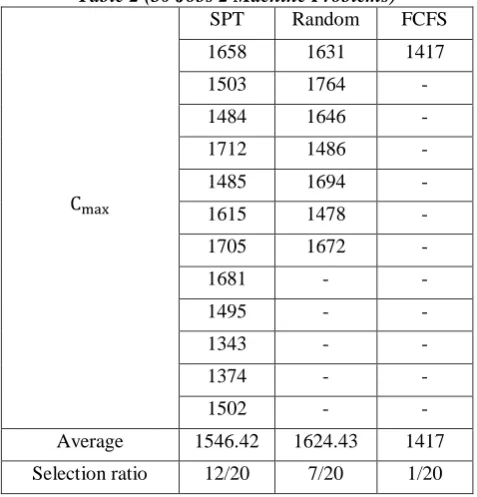
Table 2 (30 Jobs 2 Machine Problems)
Cmax
SPT Random FCFS
1658 1631 1417
1503 1764 -
1484 1646 -
1712 1486 -
1485 1694 -
1615 1478 -
1705 1672 -
1681 - -
1495 - -
1343 - -
1374 - -
1502 - -
Average 1546.42 1624.43 1417
Selection ratio 12/20 7/20 1/20
Table 2 show that the SPT rule was selected 12 times and gives average of makespan (Cmax) approximately the same for the selected two rules. Although the FCFS rule was gives the lowest average of makespan (Cmax), but this rule selected only one time from 20 runs.
Table 3 (100 Jobs 2 Machine Problems)
FCFS SPT Random
5367 4931 4888
4926 4584 5503
5187 4803 4809
[Hafez* 5(9): September, 2018] ISSN 2349-4506
Impact Factor: 3.799
G
lobal
J
ournal of
E
ngineering
S
cience and
R
esearch
M
anagement
Cmax 5242 4844 -
- 5062 -
- 5263 -
- 4805 -
- 5769 -
- 5128 -
- 4634 -
Average 5160.6 5014.91 5187
Selection ratio 5/20 11/20 4/20
Table 3 show that SPT rule was gives the lowest average of makespan (Cmax), and their selection was 11 times.
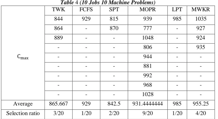
Table 4 (10 Jobs 10 Machine Problems)
Cmax
TWK FCFS SPT MOPR LPT MWKR
844 929 815 939 985 1035
864 - 870 777 - 927
889 - - 1048 - 924
- - - 806 - 935
- - - 944 - -
- - - 881 - -
- - - 992 - -
- - - 968 - -
- - - 1028 - -
Average 865.667 929 842.5 931.4444444 985 955.25
Selection ratio 3/20 1/20 2/20 9/20 1/20 4/20
Table 4 show that the MOPR rule was selected 9 times and gives average of makespan (Cmax) approximately the
same for the selected fifth rules. Although the TWK, FCFS and SPT rules were given the lowest average of makespan (Cmax), but these rules selected 3, 1 and 2 times respectively from 20 runs.
Table 5 (30 Jobs 10 Machine Problems)
Cmax
MWKR MOPR SPT
1932 1819 1936
1854 1953 -
1853 1841 -
2172 1870 -
1904 1951 -
1873 1839 -
[Hafez* 5(9): September, 2018] ISSN 2349-4506
Impact Factor: 3.799
G
lobal
J
ournal of
E
ngineering
S
cience and
R
esearch
M
anagement
1935 1964 -
- 1846 -
- 1905 -
- 1828 -
Average 1944 1880.818182 1936
Selection ratio 8/20 11/20 1/20
Table 5 show that MOPR rule was gives the lowest average of makespan (Cmax), and their selection was 11 times.
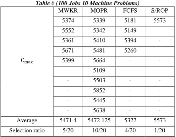
Table 6 (100 Jobs 10 Machine Problems)
Cmax
MWKR MOPR FCFS S/ROP
5374 5339 5181 5573
5552 5342 5149 -
5361 5410 5394 -
5671 5481 5260 -
5399 5664 - -
- 5109 - -
- 5503 - -
- 5852 - -
- 5445 - -
- 5638 - -
Average 5471.4 5472.125 5327 5573
Selection ratio 5/20 10/20 4/20 1/20
Table 6 show that the MOPR rule was selected 10 times and gives average of makespan (Cmax) approximately the
same for the selected three rules. Although the MWKR and FCFS rules were given the lowest average of makespan (Cmax), but these rules selected 5 and 4 times respectively from 20 runs.
Table 7 (10 Jobs 20 Machine Problems)
Cmax
MWKR SPT Random FCFS S/ROP LPT TWK LCLS MOPR
1548 1373 1387 1499 1542 1543 1460 1314 1495
1537 1406 1548 - - - 1351 1590 -
1441 - - - -
1462 - - - -
1379 - - - -
1462 - - - -
[Hafez* 5(9): September, 2018] ISSN 2349-4506
Impact Factor: 3.799
G
lobal
J
ournal of
E
ngineering
S
cience and
R
esearch
M
anagement
1555 - - - -
Average 1462.63 1389.5 1467.5 1499 1542 1543 1405.5 1452 1495
Selection ratio 8/20 2/20 2/20 1/20 1/20 1/20 2/20 2/20 1/20
Table 7 show that the MWKR rule was selected 8 times and gives average of makespan (Cmax) approximately the same for the selected eights rules. Although the SPT, TWK and LCLS rules were given the lowest average of makespan (Cmax), but these rules selected only two times from 20 runs.
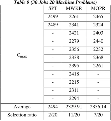
Table 8 (30 Jobs 20 Machine Problems)
Cmax
SPT MWKR MOPR
2499 2261 2465
2489 2341 2324
- 2421 2403
- 2279 2440
- 2356 2232
- 2338 2368
- 2395 2261
- 2418 -
- 2215 -
- 2311 -
- 2294 -
Average 2494 2329.91 2356.14
Selection ratio 2/20 11/20 7/20
Table 8 show that MWKR rule was gives the lowest average of makespan (Cmax), and their selection was 11 times.
Table 9 (100 Jobs 20 Machine Problems)
Cmax
MOPR MWKR SPT
5875 5589 6215
5645 6070 -
5734 6029 -
5696 5786 -
6029 5763 -
5779 5587 -
5958 5506 -
- 5796 -
- 6005 -
[Hafez* 5(9): September, 2018] ISSN 2349-4506
Impact Factor: 3.799
G
lobal
J
ournal of
E
ngineering
S
cience and
R
esearch
M
anagement
- 4865 -
- 6065 -
Average 5816.57 5753.25 6215
Selection ratio 7/20 12/20 1/20
Table 9 show that MWKR rule was gives the lowest average of makespan (Cmax), and their selection was 12 times.
CONCLUSION
From the previous results when the study used dispatching rules, the study suggests that:
In the case small size of machines (2 machines) and different sizes of jobs (10, 30 and 100), it is preferable to use SPT rule.
In the case medium size of machines (10 machines) and different sizes of jobs (10, 30 and 100), it is preferable to use MOPR rule.
In the case large size of machines (20 machines) and different sizes of jobs (10, 30 and 100), it is preferable to use MWKR rule.
In the case used dispatching rules this helps interested (business owners) on Minimize idle time this may reduce depreciation, maintenance and costs. Get the optimum time and the number of suitable machines as well as the number of jobs suitable for each machine. Saving money and effort and arrange the job flow.
REFERENCES
1. Ali, A., C.T. Ng, T.C.E. Cheng and Mikhail Y. Kovalyov (2008). “A survey of Scheduling Problems with Setup Times or Costs” European Journal of Operational Research 187 - 985–1032.
2. Dugardin F., Chehade H., Amodeo L., Yalaoui F. and Prins C. (2007)” Hybrid Job Shop and Parallel Machine Scheduling Problems: Minimization of Total Tardiness Criterion”, Multiprocessor Scheduling: Theory and Applications, Austria.
3. Gupta D., Singla S., Singla P. and Singh S.(2013) “Minimization of Elapsed Time in N×3 Flow Shop Scheduling Problem, The Processing Time Associated With Probabilities Including Transportation Time ” International Journal of Innovations in Engineering and Technology Special Issue – ICAECE.
4. Pinedo, M. (2016). Scheduling Theory, Algorithms, and Systems 5thEdition New York: Springer
International Publishing.
5. Dave M. and Choudhary K. (2016)” Job Shop Scheduling Algorithms- A Shift from Traditional Techniques to Non-Traditional Techniques” Proceedings of the 10thINDIACom; IEEE Conference ID:
37465 3rdInternational Conference on “Computing for Sustainable Global Development”, 16th-
18thMarch, New Delhi (INDIA).
6. Chiang T. C. and Fu L. C. (2007). "Using Dispatching Rules for Job Shop Scheduling with Due Date Based Objectives", International Journal of Production Research, Vol. 45, No. 14, 15 July 2007, 3245– 3262.
7. Ali, F. M. and Sawsan, S. (2012). “Study the Job Shop Scheduling by Using Modified Heuristic Rule" Eng. & Tech. Journal, Vol.30, No.19.
[Hafez* 5(9): September, 2018] ISSN 2349-4506
Impact Factor: 3.799
G
lobal
J
ournal of
E
ngineering
S
cience and
R
esearch
M
anagement
9. Kumar T. V. and Babu B. G. (2014)” Optimizing of Makespan in Job Shop Scheduling Problem: A Combined New Approach” International Journal of mechanical Engineering and robotics research ISSN 2278 – 0149 www.ijmerr.com Vol. 3, No. 2, India.
10. Zhang J., Ding G., Zou Y., Qin S. and Fu J.(2017)” Review of Job Shop Scheduling Research and its New Perspectives Under Industry 4.0” J Intell Manuf DOI 10.1007/s10845-017-1350-2 Springer Science+Business Media, LLC 2017.
11. Kaban, A. K., Othman, Z.and Rohmah, D. S. (2012)” Comparison of Dispatching rules in Job Shop Scheduling Problem Using Simulation: A Case Study” International Journal of Simulation Modelling. 3, 129-140.
12. Kagthara M.S. and Bhatt M.G. (2016). "Dispatching Rules for the Job shop Scheduling" International Journal of Darshan Institute on Engineering Research & Emerging Technologies Vol. 5, No.2.
13. Rai Siva Sai Pradeep (2016). “Optimization of Job Shop Schedules Using LEKIN® Scheduling System" International Journal of Engineering and Technical Research (IJETR) ISSN: 2321-0869 (O) 2454-4698 (P), Volume-4, Issue-2.
14. Mishra S.K.and Rao C S P (2016)” Performance Comparison of Some Evolutionary Algorithms on Job Shop Scheduling Problems” IOP Conference Series: Materials Science and Engineering 149.
15. Kumar K. K., Nagaraju D., Gayathri S. and Narayanan S. (2017)” Evaluation and Selection of Best Priority Sequencing Rule in Job Shop Scheduling using Hybrid MCDM Technique” Frontiers in Automobile and Mechanical Engineering IOP Conference Series: Materials Science and Engineering 197.
16. Syarwani M., Wahyukaton and Azizah V. E. (1978) “Scheduling Analysis and Metallurgy Testing Resource Allocation at Metallurgy Laboratory B4T Bandung” Proceeding 7th International Seminar on
Industrial Engineering and Management ISSN: 1978-774X.
17. Iringova M., Vazan P., Kotianova J., and Jurovata D. (2012) “The Comparison of Selected Priority Rules in Flexible Manufacturing System” Proceedings of the World Congress on Engineering and Computer Science Vol II WCECS 2012, October 24-26, 2012, San Francisco, USA.