INTRODUCTION
There are a few ways of describing the relative position of the individual elements of the kinematic robot mechanism. The grip an-gle elements can be used as the revolute pair; on the other hand, the movable kinematic pair involved the distance from the middle of the moving unit from the unit edge used for the movement [1, 2]. From the practical point of view, in kinematic mechanisms with the mov-ing elements, ir is most practical to describe their mutual position using the system of the so-called local coordinates system (LCS) which are firmly connected (they are moving mutually with the elements) and the current position and orientation toward the general coordinates system (GCS) of which can be easily deducted.
THE LEE ALGORITHM APPLICATION
TO AVOID OBSTACLES IN THE
ROBOT WORKING ZONE
The Lee algorithm can be used for the laby-rinth problem solving in directing individual robot trajectories. Its task is to identify the shortest trajectory between two points in the “labyrinth”. The main problems involve cre-ation of a configurcre-ation field in which the ob -stacle occurs, its evaluation and the following search for the optimal trajectory [7]. The con-figuration field is the collection of all the posi -tions that can be reached by the robot caudal effector. They are expressed in the articulated coordinates [3, 4, 9].
The configuration is the sequenced location coordinates n-tuple (q1 – qn) by which the mutu-al position and the orientation of mutu-all the arm el-ements by the effector is specifically described.
Avoiding the Obstacles in the Robot Working Zone by using
the Lee Algorithm
Naqib Daneshjo
1, Marián Kralík
2, Katka Petrovčiková
1,
Erika Dudáš Pajerská
1, Michael Paštéka
21 Faculty of Business Economics with seat in Kosice, University of Economics in Bratislava, Slovakia
2 Slovak University of Technology in Bratislava, Faculty of Mechanical Engineering, Namestie Slobody 17,
81231 Bratislava, Slovakia
* Corresponding author’s e-mail: [email protected]
ABSTRACT
Non-collision trajectories of an industrial robot are the key objective when planning its handling cycles. When the robot should move optimally, precisely and safely in each situation, it is necessary that every obstacle placed in its transition trajectory should be programmed and avoided. The optimal trajectory corresponds to choosing, if possible, the shortest and most appropriate way for the specific movement to be finished. The task of avoiding obstacles by the industrial robot in its working zone can be solved by various methods and algorithms. The paper shows the use of the kinematics SCARA as a way of avoiding obstacles by a robot in the working zone using the Lee algorithm. The configuration fields and networks are being modelled for the avoidance of obstacles together with their evaluation and the search for the shortest trajectory reflected in the robot programming.
Keywords: robot working zone, Lee algorithm, local coordinates system, general coordinates system
Volume 13, Issue 2, June 2019, pages 72–83
https://doi.org/10.12913/22998624/106239
Research Journal
Accepted: 2019.04.09Advances in Science and Technology Research Journal Vol. 13(2), 2019
The objective of the Lee algorithm applica-tion is to find the non-collision path of the robot around the obstacle. The application can be di-vided into the following steps:
1. Definition of the obstacle that needs to be avoided.
2. Configuration field creation. 3. Evaluation the configuration field. 4. Optimal trajectory identification.
The obstacle that the robot with SCARA ki-nematics has to avoid by its motion is the cuboid (H×W×L = 117×59×166 mm); its model was cre-ated using the CATIA software [6, 8].
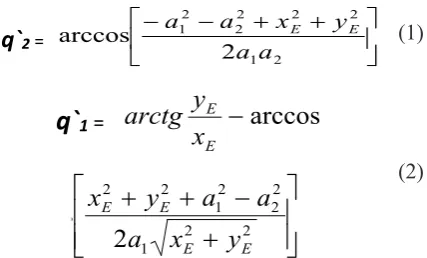
For the configuration field creation, it is nec -essary to display this obstacle in the xy plane. The configuration field is created as the dependence upon the rotation (parameter) q2 from the rota-tion (parameter) q1, the values of the both rota-tions are necessary for its creation [5, 10]. The q1 and q2 values can be acquired by using the
final formulas of the two pairs of the inverse task solution, see Figure 2.
q`
2 = 2 1 2 2 2 2 2 1 2 arccos a a y x a
a E E (1)
q`1
=
2 21 2 2 2 1 2 2
2
arccos
E E E E E Ey
x
a
a
a
y
x
x
y
arctg
q`1
=
2 21 2 2 2 1 2 2
2
arccos
E E E E E Ey
x
a
a
a
y
x
x
y
arctg
(2)While calculating the β and φ angles the value of q1 parameter can be determined:
2 2 1 2 2 2 1 2 22
arccos
E E E E E Ey
x
a
a
a
y
x
x
y
arctg
2 21 2 2 2 1 2 2
2
arccos
E E E E E Ey
x
a
a
a
y
x
x
y
arctg
(3)The q2 parameter is also calculated using the law of cosine:
2 1 2 2 2 2 2 12
arccos
a
a
y
x
a
a
E Eq
2=
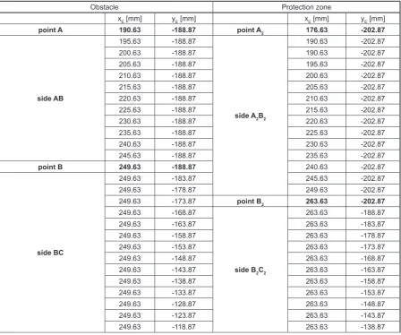
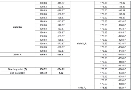
(4)size of the end robot effector; in this case – the draught tube Ø 23 mm. Table 1 also contains the points coordinates (the mutual distances in the di-rection of axis x and y equal to 5 mm as well) the so-called “protection zone” which is around each of the obstacles in the distance of 14 mm from each of its sides. Together with the obstacle co-ordinates and its protection zone, Table 1 defines the position of the starting and the end point of the robot trajectory in the xy plane.
Configuration field creation – network creation in which the obstacle is placed
The configuration field creation denotes the network creation in which the obstacle is placed. The configuration field itself is created as the dependence of the rotation (parameter) q2 to the rotation (parameter) q1. Thus, the main task is to calculate the values of both rotations for the points presenting the obstacle and its protection zone, so that its position in the configuration field
is clearly defined. The values for q1 a q2 are ac-quired using the final formulas of the two pairs of inverse task solution. These are pairs of for-mulas – the first are the forfor-mulas (1) and (2) and the second are the formulas (3) and (4). The input data are x and y coordinates from Table 1 and the values a1 and a2 are the lengths of the robot’s arms (a1 = 225 mm, a2 = 166.1 mm). The calculation results are the two solutions of the obstacle place-ment and its protection zone in the configuration field (see Table 3).
For both solutions it is necessary to construct, within the configuration point, the network of those configurations. Each solution has its own configuration field due to the choice of different increases in the direction of the axis q1 and q2 (in-creases are shown in the Table 2).
Defining the distances of the individual axes in the network is important for the precise deter-mination of the q1 and q2 rotation values of indi-vidual configurations (network points) because af -ter identifying the optimal trajectory, these values
Table 1. Coordinates for the obstacle points, protection zone, starting and end trajectory points
Obstacle Protection zone
xE [mm] yE [mm] xE [mm] yE [mm]
point A 190.63 -188.87 point A2 176.63 -202.87
side AB
195.63 -188.87
side A2B2
190.63 -202.87
200.63 -188.87 190.63 -202.87
205.63 -188.87 195.63 -202.87
210.63 -188.87 200.63 -202.87
215.63 -188.87 205.63 -202.87
220.63 -188.87 210.63 -202.87
225.63 -188.87 215.63 -202.87
230.63 -188.87 220.63 -202.87
235.63 -188.87 225.63 -202.87
240.63 -188.87 230.63 -202.87
245.63 -188.87 235.63 -202.87
point B 249.63 -188.87 240.63 -202.87
side BC
249.63 -183.87 245.63 -202.87
249.63 -178.87 249.63 -202.87
249.63 -173.87 point B2 263.63 -202.87
249.63 -168.87
side B2C2
263.63 -188.87
249.63 -163.87 263.63 -183.87
249.63 -158.87 263.63 -178.87
249.63 -153.87 263.63 -173.87
249.63 -148.87 263.63 -168.87
249.63 -143.87 263.63 -163.87
249.63 -138.87 263.63 -158.87
249.63 -133.87 263.63 -153.87
249.63 -128.87 263.63 -148.87
249.63 -123.87 263.63 -143.87
side BC
249.63 -113.87
side B2C2
263.63 -133.87
249.63 -108.87 263.63 -128.87
249.63 -103.87 263.63 -123.87
249.63 -98.87 263.63 -118.87
249.63 -93.87 263.63 -113.87
249.63 -88.87 263.63 -108.87
249.63 -83.87 263.63 -103.87
249.63 -78.87 263.63 -98.87
249.63 -73.87 263.63 -93.87
249.63 -68.87 263.63 -88.87
249.63 -63.87 263.63 -83.87
249.63 -58.87 263.63 -78.87
249.63 -53.87 263.63 -73.87
249.63 -48.87 263.63 -68.87
249.63 -43.87 263.63 -63.87
249.63 -38.87 263.63 -58.87
249.63 -33.87 263.63 -53.87
249.63 -28.87 263.63 -48.87
Point C 249.63 -22.87 263.63 -43.87
side CD
245.63 -22.87 263.63 -38.87
240.63 -22.87 263.63 -33.87
235.63 -22.87 263.63 -28.87
230.63 -22.87 263.63 -22.87
225.63 -22.87 point C2 263.63 -8.87
220.63 -22.87
side C2D2
249.63 -8.87
215.63 -22.87 245.63 -8.87
210.63 -22.87 240.63 -8.87
205.63 -22.87 235.63 -8.87
200.63 -22.87 230.63 -8.87
195.63 -22.87 225.63 -8.87
point D 190.63 -22.87 220.63 -8.87
side DA
190.63 -28.87 215.63 -8.87
190.63 -33.87 210.63 -8.87
190.63 -38.87 205.63 -8.87
190.63 -43.87 200.63 -8.87
190.63 -48.87 195.63 -8.87
190.63 -53.87 190.63 -8.87
190.63 -58.87 point D2 176.63 -8.87
190.63 -63.87
side D2A2
176.63 -22.87
190.63 -68.87 176.63 -28.87
190.63 -73.87 176.63 -33.87
190.63 -78.87 176.63 -38.87
190.63 -83.87 176.63 -43.87
190.63 -88.87 176.63 -48.87
190.63 -93.87 176.63 -53.87
190.63 -98.87 176.63 -58.87
190.63 -103.87 176.63 -63.87
190.63 -108.87 176.63 -68.87
are used for the coordinate points calculation employed in programming the robot trajectory.
Configuration field evaluation
In this step, the evaluation of the both fields will be provided in the following sequence: 1. All empty (non-collision) configura
-tions form the configuration field.
2. The starting position has 0 value.
3. All neighbouring configurations with the start -ing configuration will be given the value of 1. 4. All other non-valued configurations
neighbouring with those with val-ue 1 will be given the valval-ue of 2. 5. The configurations evaluations are run
till the final configuration is reached. side DA
190.63 -118.87
side D2A2
176.63 -78.87
190.63 -123.87 176.63 -83.87
190.63 -128.87 176.63 -88.87
190.63 -133.87 176.63 -93.87
190.63 -138.87 176.63 -98.87
190.63 -143.87 176.63 -103.87
190.63 -148.87 176.63 -108.87
190.63 -153.87 176.63 -113.87
190.63 -158.87 176.63 -118.87
190.63 -163.87 176.63 -123.87
190.63 -168.87 176.63 -128.87
190.63 -173.87 176.63 -133.87
190.63 -178.87 176.63 -138.87
190.63 -183.87 176.63 -143.87
point A 190.63 -188.87 176.63 -148.87
176.63 -153.87
176.63 -158.87
176.63 -163.87
Starting point (Z) 156.72 -204.02 176.63 -168.87
End point (C ) 256.72 -4.02 176.63 -173.87
176.63 -178.87
176.63 -183.87
176.63 -188.87
side A2 176.63 -202.87
In this way, the valued configuration fields which are suitable for the search of the trajec-tory avoiding the obstacle will be acquired (see Figures 7 and 8).
THE NON-COLLISION TRAJECTORY
IDENTIFICATION FOR THE ROBOT
AVOIDING THE OBSTACLE
The aim of this step is to identify one or more paths that are non-colliding for the robot; mean-ing they avoid the obstacle. Identification is done in a different direction than the configuration field evaluation in the following steps:
1. From the configurations adjacent to the end configuration, the one with the lowest value is selected.
2. From the configurations adjacent to this con -figuration, only the one with the lowest value is selected again.
The configuration selected carried out in this way till the starting configuration is reached.
In this case, we were searching for the two path types – the closest one to the obstacle and the closest path to the obstacle with the lowest
number of the cranks in the used configuration field. While searching the paths in the configura -tion field, it is important to take into considera-tion that the distance between the two adjacent con-figurations is constant also in terms of the values of the rotations q1 or q2. In the case of program-ming the coordinates of x and y, it is impossible to talk about the constant distance of the adjacent configurations because for their calculations, the cosine and sinusoidal formulas are applied for the sum of the rotations. This fact causes irregular changes in the coordinates x and y values when changing the values of the rotations q1and q2 by the constant figure. This is the reason to identify two different path types for each solution which are later compared according to their length with the aim to find the shortest one.
As we can see in Figure 7, the numeric value of the target point has the same value 40 after the field evaluation around the obstacle from above and under. That is the reason why 4 trajectories were found for the 1st solution (two closest to the
obstacles and two closest to the obstacles with the lowest number of the cranks). Figure 8 shows that in the second solution, the maximum value of the numeration the target point 37 is reached while evaluating the field around the obstacle. There -fore, 2 trajectories were found for the second so-lution – one is the closest one to the obstacle and the second is the closest one to the obstacle with the lowest number of the cranks. All the identi-fied trajectories (6 together) are shown in Fig -ures 9 to 12 (the trajectories are shown in red or blue double line).
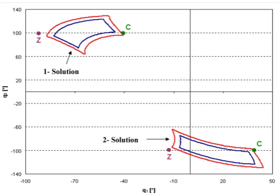
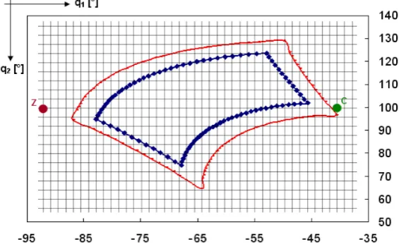
Figure 4 Image of the obstacle and the protection zone in the configuration field
(The blue line – the obstacle, The red line – the protection zone, Z – the starting point, C – the end point)
Table 2 Increases in the rotations q1 and q2 for the first and second solution
Δ q1 [°] Δ q2 [°]
1st solution 1.33 4
Transformation of the rotation values of q1 and q2 to x and y coordinates
The configuration field is formed as the de -pendence of the rotations q2 from q1; so the in-dividual configurations (points, the configuration nodes) are defined by these two parameters. In the case of programming, it is better to know the x and y coordinates of the points because it is easier to load them to the robot Central Processing Unit. In order to do this, it is necessary for the each point of the identified trajectories in the configuration field to execute the transformation (recalculation) of the rotation q1 and q2 values to the values of the coordinates x and y. the recalculation of the rota -tions to the coordinates of the point on the plane
xy will be done using the formulas (5) and (6) that are derived from the final transformation matrix TE (see Figure 13). The input data are the rota-tions q1 and q2 and the length values of the robot arms (a1 = 225 mm, a2 = 166.1 mm).
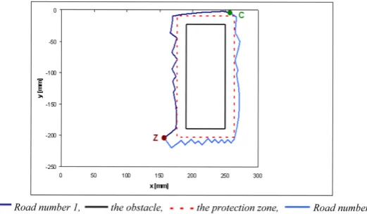
After the calculation of the point coordinates x, y of the found trajectories, it is possible to dis -play those trajectories together with the avoiding obstacle and its protection zone in the xy plane. Figures 15 and 16 show the trajectories stemming from Figure 9 and Figure 10 (the identified tra -jectories closest to the obstacle and the trajectory closest to the obstacle with the lowest number of the cranks for the 1st solution of the obstacle
posi-tion in the configuraposi-tion field).
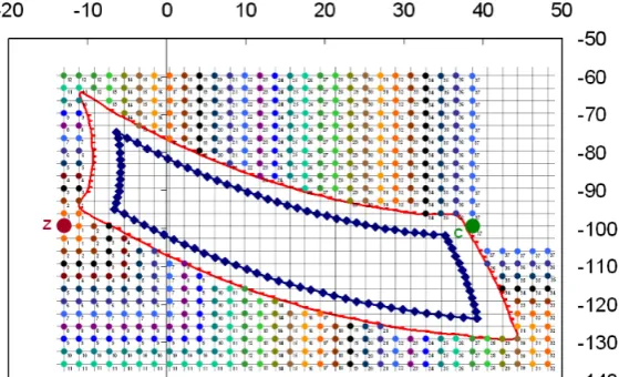
Figure 5 Configuration field together with the displayed configuration network for the 1st solution for the obstacle and its protection zone position in the field:
(The blue line – the obstacle, The red line – the protection zone, Z – the starting point, C – the end point)
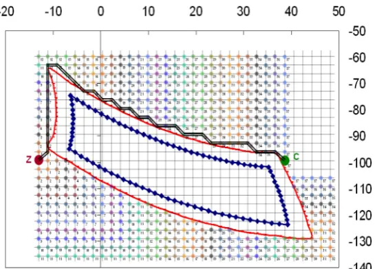
Figure 6 Configuration field together with the displayed configuration network for the 2nd solution for the obstacle and its protection zone position in the field:
Figures 17 and 18 show the identified tra -jectories for the 2nd solution of the obstacle
po-sition in the configuration field stemming from figures 11 and 12 (the closest trajectory to the ob -stacle and the closest trajectory with the lowest number of the cranks).
DISCUSSION
After the Lee algorithm application for the determination of the few trajectories of the robot movement around the defined obstacle and the coordinates x, y calculation of the single points of the identified trajectories, it is possible to create the robot’s manipulation motion programs. The robot used by us is Robot Yamaha YK400K and is programmed in the on-line regime directly by manual controlling unit.
There are 6 programs for the controlling of the robot manipulating movement – 1 for each
programming is continuous without any inter-ruption, so it is the continuous path of the robot movement. (continuous path – CP). While pro-gramming a robot, the following steps are taken: 1. The obstacle is placed in the robot’s working
area – its position as well as the position of the initial and the target motion point are known (see Table 1),
2. Loading of the coordinates’ points forming the trajectory for the robot movement together with the starting and the end motion point into the robot controlling unit,
3. Creation of the robot program motion itself, 4. Verification of the obstacle avoidance
programme,
5. Implementation of the created programme for the obstacle avoidance.
The trajectories are compared in relation to the economics of the manipulation cycles from the two Figure 8 The evaluated configuration field for the 2nd solution for the obstacle position
For the length of the identified trajectories around the obstacle, the Pythagoras’ theorem is used. The calculated lengths are shown in the Table 3.
The comparing of the trajectories according to the time is allowed due to the same position
of the starting and the end motion point as well as by the compliance with the executing and the number of the ongoing commands in all six pro -grammes for the robot motion. The measured val-ues are defined in the Table 4.
Figure 11 The identified trajectory closest to the obstacle for the 2nd solution of the obstacle position Figure 9 The identified trajectories closest to the obstacle for the 1st solution of the obstacle position
Figure 14 The image of the robot arm SCARA in the xy plane for the q1 and q2 parameter calculation
Figure 15 Display of the of the identified trajectories closest to the obstacle for the 1st so-Figure 12 The identified trajectory closest to the obstacle with the lowest number of the cranks
for the 2nd solution of the obstacle position
Figure 16 Display of the identified trajectories closest to the obstacle with the lowest num -ber of the cranks for the 1st solution of the obstacle position in the configuration field
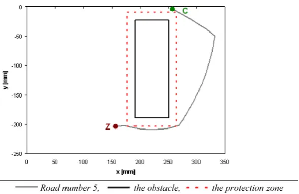
Figure 17 Display of the of the identified trajectories closest to the obstacle for the 2nd so-lution of the obstacle position in the configuration field in the xy plane
On the basis of the acquired data on the robot movement trajectory length and on the time length of its movement, it can be stated that trajectory No. 3 is optimal regarding both aspects (see Figure 15).
CONCLUSION
The planning of the robot’s manipulation cy-cles is one of the key problems in the robot tech-nology area. It is the security, appropriateness, non-collision and accuracy solution for the projected motion trajectory. The avoidance of obstacles and thus ensuring the safe and economic motion of an industrial robot in the application environment are the programming priority. There are few methods to prevent the robot’s collision or more precisely its end effector with the obstacle and to ensure si -multaneous economy of the manipulation cycles.
The Lee algorithm is quite a simple solution of securing the non-collision motion of the industrial robot around the obstacle which position in the working area of the robot is known. It is one of the methods that combine the computerized and graph-ic elements to specify the non-collision motion tra-jectory of the industrial robot. It suitably combines the kinematic robot structure and the transforma-tion matrices calculatransforma-tion with the graphic search for the trajectory avoiding the obstacle in the robot configuration field. Performing all the necessary calculation, creating the configuration field, evalu -ating it and identifying the non-collision industrial model motion trajectory requires a lot of time for the programmer. However, the Lee algorithm still has its place among the more exact used methods of solving the problem of the obstacle avoidance in the robot working area at the workplace.
Acknowledgements
This work was supported by the Slovak Re-search and Development Agency under the con-tract No. APVV-16–0485 and VEGA 1/0376/17.
REFERENCES
1. Angeles J.: Fundamentals of Robotic Mechanical Systems (Theory, Methods, and Algorithms) Montreal. Springer, 2007.
2. Ceng J., Krämer S.: OOP-Project Maze Router with Lee Algorithm. Aachen. Institute for Integrated Signal Processing Systems, 2007.
3. Daneshjo N., Králik M., Majerník M., Dudáš Pajerská E., Naščáková J.: Non-collision trajec -tories of service industrial robots. Advances in Engineering Software, 124 (2018), 90–96.
4. Daneshjo N., Korba P., Vargová R., Tahzib B. Application of 3D Modeling and Simulation Using Modular Components. Applied Mechanics and Materials, 389 (2013), 957–962.
5. Gálisová L., Knežo D.: Macroscopic ground-state degeneracy and magnetocaloric effect in the ex -actly solvable spin-12 Ising-Heisenberg double-tetrahedral chain. Physics Letters A. 39 (2018), 2839–2845.
6. Knežo, D., Andrejiová, M., Kimáková, Z., Radchenko, S.: Determining of the optimal device lifetime using mathematical renewal models. TEM Journal. 2 (2016), 121–125.
7. Manová E., Čulková K., Lukáč J., Simonidesová J., Kudlová J.: Position of the Chosen Industrial Companies in Connection to the Mining. Acta Montanistica Slovaca. Košice. Technical University of Košice, 23(2018), 132–140.
8. Palko A., Smrček J.: The use of pneumatic ar -tificial muscles in robot construction. Industrial Robot – An International Journal. 1 (2011), 11–19.
9. Pribulová A., Futáš P., Petrík J., Pokusová M., Brzezinski, M., Jakubski, J.: Comparison of cu-pola furnace and blast furnace slags with respect to possibilities of their utilization. Archives of Metallurgy and Materials. 4 (2018), 1865–1873. 10. Semjon J., Sukop M., Vagaš M., Jánoš R.,
Tuleja P., Koukolová L., Marcinko P., Juruš O., Varga J.: Comparison of the delta ro-bot ABB IRB 360 properties after collisions. Communications – Scientific Letters of the University of Zilina. 1 (2018), 42–46.
Table 4 Times of the robot motion while avoiding the obstacle
Trajectory No. 1 Trajectory No. 2 Trajectory No. 3 Trajectory No. 4 Trajectory No. 5 Trajectory No. 6
Time [s] 29.47 32.67 29.11 33.79 31.36 32.49
Table 3 The lengths of the identified trajectories for the robot obstacle avoidance
Trajectory No. 1 Trajectory No. 2 Trajectory No. 3 Trajectory No. 4 Trajectory No. 5 Trajectory No. 6 Leght of the