30
Two-Group MultiODA: A Mixed-Integer
Linear Programming Solution with
Bounded
M
Robert C. Soltysik, M.S., and Paul R. Yarnold, Ph.D.
Optimal Data Analysis, LLCPrior mixed-integer linear programming procedures for obtaining two-group multivariable optimal discriminant analysis (Multi-ODA) models require estimation of the value of a parameter, M. A new formulation is presented which establishes a lower bound for
M, which executes more quickly than prior formulations. A suf-ficient condition for the nonexistence of classification gaps and ambiguous solutions, optimal weighted classification, use of non-linear terms, selecting an optimal subset of attributes, and aggre-gation of duplicate observations are discussed. When the design involves six or fewer binary attributes, MultiODA models may easily be obtained for massive samples.
.
Classification models derived via multivariable optimal discriminant analysis (MultiODA) are linear discriminant classifiers which explicitly maximize classification accuracy for a given sample.1 Mixed-integer linear programming formulations for two-group MultiODA models require estimation of the value of a parameter,
M, commonly defined as “a prohibitively large number.”2 If the estimated value of M is too low then suboptimal solutions may occur, and exces-sively large values of M will decrease computa-tional efficiency and may introduce numerical (round-off) error.3 We present a goal program-ming formulation which establishes a lower bound for M, and then we discuss a sufficient condition for the nonexistence of classification gaps and ambiguous solutions, weighted classi-fication, the use of nonlinear terms, selection of
optimal subsets of attributes, and aggregation of duplicate observations.
MIP45 Methodology
In a two-group linear MultiODA problem with p attributes and m observations, a set of m
31
minimize the number of misclassified observa-tions. This is achieved by determining x* which satisfy the maximum number of inequalities in the system:
aix < 0 for observations in class 0,
aix > 0 for observations in class 1. (1)
This problem may be formulated as a mixed-integer linear programming model. To accomplish this, the strict inequalities in (1) are replaced with aix < - or aix > , where > 0. This is necessary due to the inability of simplex-based algorithms for mixed-integer program-ming to handle strict inequalities (mixed-integer techniques based upon interior-point algorithms4 may not suffer this limitation). Letting be strictly positive removes the ambiguity in the classification status of observations i for which aix = 0, but also introduces the possibility of a classification gap. It will be shown that there are conditions under which ambiguities can be re-moved for = 0. Consider the following model: m MIP45: z = min di (2)
i=1 subject to n aij (xj+ - xj-) - Midi -, i I0 (3)
j=1 n aij (xj+ - xj-) + Midi, i I1 (4)
j=1 n (xj+ + xj-) = 1 (5)
j=1 xj+ - gj 0, j=1,..., n (6)
xj- + gj 1, j=1,..., n (7)
xj+, xj- 0, j=1,..., n (8)
gj {0,1}, j=1,..., n (9)
di {0,1}, i=1,...,m (10)
where aij is the jth component of observation ai I0 is the set of observations belonging to class 0 I1 is the set of observations belonging to class 1 Mi = max aij + (11)
j z is the number of misclassified observations. The weight vector x is obtained by xj = xj+ - xj-, j=1,..., n. (12)
Since constraints (6) and (7) ensure that not more than one of the xj+ and xj- are positive for any j, we can think of these values as the "pos-itive" and "negative" parts of xj, respectively. Note that gj = 1 when xj > 0 and gj = 0 when xj < 0. Also note that the gj, along with (6), (7), and (9), may be dropped when > 0. Constraint (5) normalizes x so that n xj = 1 ; (13) j=1
32
aix - max aij (14)
j
and
aix + max aij + . (15)
j
Therefore, when di = 1,
aix + Midi. (16)
Because the normalization (5) requires that all optimal weight vectors x* lie on a 45° properly rotated hypercube centered at the origin, this formulation is referred to as MIP45. It may be the case that more than one solution for d may be optimal for a problem. This cor-responds to the existence of multiple optimal dichotomies of predicted class membership. It is also generally true that a solution space for x of positive volume exists for each dichotomy. The issue of selecting among optimal x* may be addressed by a number of methods, such as linear programming5 and a priori decision heuristics.6
Resolving Classification Gaps and Ambiguities
In the above formulation, at least n - 1 of the aix* are at zero when = 0 is specified. From (1), it is seen that the criterion of strict separation of the classes should be met. An optimal value z* > 0 in the solution of the following linear program guarantees that this separation is maintained.
LP: max z = y
subject to
n
aij (bj+ - bj-) + y 0, i I0 and aix* 0 j=1
(17)
n
aij (bj+ - bj-) - y 0, i I1 and aix* 0 j=1
(18)
n
(bj+ - bj-) = 1 (19) j=1
bj+, bj-, y 0 (20)
bj = bj+ + bj- . (21)
This LP may be executed for each optimal dichotomy. If z* > 0 is obtained, b* is a new discriminant vector which optimizes criterion (1). Otherwise, ambiguity remains in the class-ification status of observations for which aib* = 0: such observations should not be classified. The advantage of establishing a lower bound for M is illustrated with an example in-volving discriminating between excellent versus less than excellent medical residents using information obtained during their application for residency training. Since rating applicants for residency training is a difficult, time-intensive decision-making task, a linear discriminant classifier that successfully predicts resident performance might be of great interest and utility to admissions committees.
33
and academic distinction (a composite measure reflecting honors attained in medical school and medical school status).
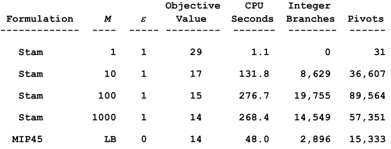
The computer resources required to solve this problem using MIP45 versus Stam and Joachimsthaler8 was compared (other prior for-mulations were slower). For MIP45, was set at 0. For Stam and Joachimsthaler, values of 1, 10, 100, and 1000 were used for M, and a value of 1 for .9 All formulations were solved on an IBM 3090/300 computer running SAS/OR.10 As seen in Table 1, except when M = 1, Stam and Joachimsthaler required more computa-tional effort (CPU time, pivots, and integer
branches) than did MIP45. Using M = 1, = 1 in Stam and Joachimsthaler resulted in a useless solution, and using M = 10 or 100 resulted in suboptimal solutions of (3). Since a decision-maker using M = 10 or M = 100 would have no direct evidence that these solutions were sub-optimal, it would also be unclear whether the solution attained by Stam and Joachimsthaler (or other unbounded formulations) using M = 1000 was optimal. In contrast, since the value of z* attained in LP was positive, a decision-maker using MIP45 to solve this problem would be certain that the solution was unambiguously optimal: a clear advantage.
TABLE 1
Illustration of Computational Resources Needed by MIP45 Versus Stam and Joachimsthaler8 to Solve a Problem with 49 Observations and Three
Attributes, Using SAS/OR run on an IBM 3090/300 Computer
Objective CPU Integer
Formulation M Value Seconds Branches Pivots --- ---- --- --- --- --- ---
Stam 1 1 29 1.1 0 31
Stam 10 1 17 131.8 8,629 36,607
Stam 100 1 15 276.7 19,755 89,564
Stam 1000 1 14 268.4 14,549 57,351
MIP45 LB 0 14 48.0 2,896 15,333 --- Note: For MIP45 the Mi were set at their lower bounds (LB). For solutions resulting in the optimal value of 14 misclassifications, model coefficients for board scores and faculty evaluation were positive, and the coefficient for academic distinction was negative. For MIP45, z* = .00439.
Weighted Classification
Rather than weighting each observation equally, we consider weighting each case in (2) by a positive scalar ci. This is significant for two reasons. First, the ci may represent the cost of misclassifying observation i. In this case an
34
correct classifications weighted by population membership in each class. An example would be ci = 1/m0 for observations in class 0, and ci = 1/m1 for observations in class 1, where m0 and
m1 are the number of observations in categories 0 and 1, respectively. This latter weighting scheme is particularly useful in badly imbalanced applications for which m0 >> m1, or visa versa: use of such “priors weights” forces the model to classify observations from both classes accurately, and inhibits the identification of degenerate models which classify all observations into a single class category.
Adding Nonlinear Terms as Attributes
Here we generalize the notion of maximum pattern classification accuracy achieved by separating hyperplanes to sets of nonlinear separating surfaces. For example, consider quadratic surfaces in p-measurement space of the form:
aij xj + aikailxkl + ainxn (22) j kp l < k
for all i. The MultiODA solution can be attain-ed by augmenting the aj and x in the MIP45 model by the interaction terms in (22). This solution produces a weight vector x which yields the minimum number of misclassifica-tions achievable by a quadratic separating surface. This process may be applied to any nonlinear discriminant function which is linear in the parameters of the measurement space.
Optimal Attribute Subset Selection
In the foregoing we have assumed that all p
attributes are included in the MultiODA model. However, we may wish to select a subset of k <
p attributes for the application of the model. For example, imagine an application involving 50 observations and ten attributes. In order to identify a model that may generalize if used to classify independent random samples, we may wish to maintain a minimum
observation-to-attribute ratio of 10-to-1, so a maximum of five of the ten potential attributes may be used. Of all possible 5-attribute models, which yields maximum accuracy? Optimal attribute subset selection methodology can be incorporated in the MIP45 model by defining n zero-one var-iables qj and including the following constraints:
xj- - qj < 0, j=1,..., n, (23) gj + qj < 1, j=1,..., n, (24)
and
n n
gj + qj = k. (25) j = 1 j = 1
In an optimal solution to such a MultiODA model, measurement j is selected for inclusion only if gj + qj = 1. The number of misclassifica-tions obtained is the fewest achievable in any k -dimensional subspace of the original p -dimen-sional measurement space.
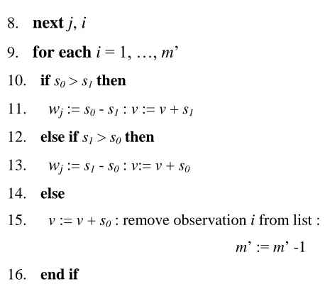
Aggregation of Duplicate Observations
If duplicate observations occur in the data set (i.e., two or more observations have the same value for every attribute measurement), the following procedure may be used to aggregate the duplicate observations into a single observation, reducing the size of the overall problem. The resulting problem is equivalent to the original one, with m’
observa-tions, and objective value z + v.
1. m’ := m : s0 = 0: s1 = 0: v := 0
2. for eachi = 1, …, m’
3. for eachj < i
4. ifai = ajthen
5. ifi I0 thens0 := s0 + cielses1 := s1 + ci 6. remove observation i from list : m’ := m’ - 1
35
8. next j, i
9. for eachi = 1, …, m’
10. ifs0 > s1then
11. wj := s0 - s1 : v := v + s1
12. else ifs1 > s0then
13. wj := s1 - s0 : v:= v + s0
14. else
15. v := v + s0 : remove observation i from list :
m’ := m’ -1
16. end if
17. next i
This procedure is particularly useful when aj is a zero-one vector (all attributes are binary). Here all the patterns lie on the vertices of the p -dimensional unit hypercube. If more than one pattern lies on some vertex, then by using the above procedure we may obtain a weighted MIP45 model equivalent to the original model, but with fewer constraints. If the number of original patterns m is large relative to the number of attributes p, a significant reduction in the size of the model may be obtained. For instance, regardless of the value of m, if p=8 then we end up with no more than 28 = 256 constraints of type (6) in the model. Since the number of constraints is independent of m, extremely large problems may be solved with this procedure, provided p is moderately small.
In order to illustrate the potential solution efficiency gained by using this special purpose algorithm for problems involving entirely binary data, we ran 30 Monte Carlo experiments. In each experiment there were five binary attributes, such that the total possible number of different profiles was 25 = 32. Values on each attribute were determined separately for each observation on the basis of a random uniform number between 0 and 1: numbers < 0.5 were assigned the value of 0, and numbers > 0.5 were assigned the value of 1. We ran five balanced (m0 = m1) experiments for each total sample size of 50, 100, 1000, 104, 105, and 106 total observa-tions. All formulations were solved on an IBM 3090/300 computer running SAS/OR. As seen in Table 2, as the number of observations increased: (a) the number of distinct profiles increased toward its theoretical upper bound (the theoretical upper bound was achieved in all of the problems involving 106 observations, and in four of the five problems involving 105 observations); (b) the misclassification rate increased towards its theoretical upper bound (i.e., for a balanced design with an even number of observations, the theoretical upper bound for the number of misclassifications is one less than one-half of the total number of observations); and (c) the mean number of CPU seconds required to solve the problem was approx-imately twenty seconds for problems with 1000 or more total observations.
TABLE 2
Results of Monte Carlo Experiments for Binary Data: Five Random Attributes
Number of Number of Number (%) of CPU Observations Profiles Misclassifications Seconds
36
50 23 14 (28%) 12.5 50 21 12 (24%) 1.7
100 30 27 (27%) 14.2 100 26 34 (34%) 9.0 100 25 43 (43%) 10.5 100 24 37 (37%) 7.5 100 20 33 (33%) 3.0
1000 32 432 (43%) 17.8 1000 30 445 (44%) 25.1 1000 31 449 (45%) 16.4 1000 31 460 (46%) 24.3 1000 31 454 (45%) 19.2
10000 29 4870 (49%) 12.3 10000 31 4838 (48%) 23.8 10000 31 4842 (48%) 24.9 10000 29 4828 (48%) 11.9 10000 31 4839 (48%) 9.2
100000 32 49545 (50%) 14.5 100000 32 49532 (50%) 21.6 100000 31 49526 (50%) 6.3 100000 32 49475 (49%) 25.2 100000 32 49376 (49%) 16.8
1000000 32 498331 (50%) 24.3 1000000 32 498759 (50%) 17.2 1000000 32 498450 (50%) 32.5 1000000 32 497861 (50%) 4.5 1000000 32 498837 (50%) 16.8 ---
Discussion
MIP45 solves two problems common to prior goal programming formulations of two-group MultiODA: M is automatically set at its lower bound, and it is possible to determine whether classification gaps or ambiguities exist. Collateral benefits of MIP45 include its greater computational efficiency and solution speed relative to prior formulations, particularly for applications involving binary attributes.
37
irreducible inconsistent subsystems (IIS) of linear inequalities in order to determine a maxi-mum feasible subsystem of these inequalities.13 Finally, Bremner and Chen developed a MIP formulation for the halfspace depth problem which uses IIS cuts in a branch-and-cut algor-ithm.14 We eagerly anticipate computational comparisons between these formulations.
References
1
Yarnold PR, Soltysik RC, Martin GJ. Heart rate variability and susceptibility for sudden car-diac death: an example of multivariable optimal discriminant analysis. Statistics in Medicine
1994, 13:1015-1021.
2
Joachimsthaler EA, Stam A. Mathematical programming approaches for the classification problem in two-group discriminant analysis.
Multivariate Behavioral Research 1990,
25:427-454.
3
Gehrlein WV. General mathematical program-ming formulations for the statistical classifica-tion problem. Operations Research Letters
1986, 5:299-304.
4
Karmarkar N. A new polynomial time algor-ithm for linear programming. Combinatorica
1984, 4:373-395.
5
Koehler GJ, Erenguc SS. Minimizing mis-classifications in linear discriminant analysis.
Decision Sciences 1990, 21:63-74.
6
Yarnold PR, Soltysik RC. Theoretical distribu-tions of optima for univariate discrimination of random data. Decision Sciences 1991, 22:739-752.
7
Curry RH, Yarnold PR, Bryant FB, Martin GJ, Hughes RL. A path analysis of medical school and residency performance: implications for housestaff selection. Evaluation in the Health
Professions 1988, 11:113-129.
8
Stam A, Joachimsthaler EA. A comparison of a robust mixed-integer approach to existing methods for establishing classification rules for the discriminant problem. European Journal of
Operational Research 1990, 46:113-122.
9
Bajgier SM, Hill AV. An experimental com-parison of statistical and linear programming approaches to the discriminant problem.
Decis-ion Sciences 1982, 13:604-612.
10
Cornell R, Luginbuhl RC, Yeo C. SAS/OR
user’s guide, version 6. SAS Institute, Durham,
NC, 1989.
11
Rubin PA. Solving mixed-integer classifica-tion problems by decomposiclassifica-tion. Annals of
Operations Research 1997, 74:51-64.
12
Silva APD, Stam A. A mixed-integer pro-gramming algorithm for minimizing the training sample misclassification cost in two-group classification. Annals of Operations Research
1997, 74:129-157.
13
Pfetsch ME. Branch-and-cut for the maxi-mum feasible subsystem problem. SIAM
Jour-nal on Optimization 2008, 19:21-38.
14
Bremner D, Chen D. A branch and cut algor-ithm for the halfspace depth problem. 2009: arXiv:0910.1923v1.
Author Notes