Numerical analysis via Chebyshev pseudospectral method for nonlinear initial/boundary value problems

J. Math. Comput. Sci. 6 (2016), No. 4, 597-619 ISSN: 1927-5307

NUMERICAL ANALYSIS VIA CHEBYSHEV PSEUDOSPECTRAL METHOD FOR NONLINEAR INITIAL/BOUNDARY VALUE PROBLEMS

NADER Y. ABD ELAZEM, ABDELHALIM EBAID∗

Department of Mathematics, Faculty of Science, University of Tabuk, Tabuk 71491, Saudi Arabia

Copyright c2016 Abd Elazem and Ebaid. This is an open access article distributed under the Creative Commons Attribution License, which permits unrestricted use, distribution, and reproduction in any medium, provided the original work is properly cited.

Abstract.In applied science, the physical models are usually described by nonlinear initial/boundary value prob-lems. The exact solutions for such nonlinear models are not always available, the reason that many authors resort to the numerical methods. One of these numerical methods is the Chebyshev pseudospectral method. This method is applied in the current paper to solve some nonlinear initial and boundary value problems of particular interest in applied sciences and engineering. In order to explore the effectiveness and the validity of the present method, many physical models of nonlinear type such as generalized nonlinear oscillator, relativistic oscillator, and Bratu’s equations have been solved numerically. The obtained results are compared with other published works through tables and graphs where good accuracy has been achieved.

Keywords: Chebyshev collocation method; Nonlinear oscillator; Initial and boundary value problems; Bratu’s problem.

2010 AMS Subject Classification:35G31, 65L05.

1. Introduction

Physical models in applied mathematics and engineering sciences are usually formulated as nonlinear initial or boundary value problems. The exact solutions of such models can not be obtained in the most cases, especially, when the considered model is of complex nonlinearity.

∗_{Corresponding author}

Received August 23, 2014

598 NADER Y. ABD ELAZEM, ABDELHALIM EBAID

Because of the difficulty of obtaining the exact solution for nonlinear differential equations with complex nonlinearities, many mathematicians resort to one of the efficient numerical method-s. Chebyshev have proven successfully in the numerical solution of various boundary value problems [1,2] and in computational fluid problems [3,4]. The spectral method distinguishes itself from the finite-difference and finite-element methods by the fact that global information is incorporated in computing a spatial derivative. The spectral method can yield greater accu-racy for a smooth solution with far fewer nodes and therefore less computational time than the finite-difference and finite-element schemes [5].

Chebyshev pseudospectral methods are widely used in the numerical approximation of many types of ordinary and partial differential equations which arise from the engineering problem-s [6-9]. Therefore, when many decimal placeproblem-s of accuracy are needed, the conteproblem-st between pseudospectral algorithms and finite difference is not an even battle but a rout: pseudospectral methods win hands-down. Moreover, engineers and mathematicians who need accurate many decimal places have always preferred spectral methods [10]. Elbarbary and El-Sayed [11-13] has recently introduced a new pseudospectral differentiation matrix to decrease the round off error, specially on increasingN(the number of degrees of freedom) or number of equations.

Wazwaz [23] discussed A domian decomposition method for a reliable treatment of the Bratu-type equations. An efficient computational method for second order boundary value problems was studied by Zhou et al. [24].

The purpose of this work is to study the applicability of the Chebyshev collocation method to solve this kind of issues; see [10, 15, 16, 18, 21, 22, 23]. The absolute errors of the present results are compared with those obtained by other methods. The nonlinear oscillator with both initial and boundary conditions is investigated in this paper utilizing Chebyshev collocation method. It is hoped that the results obtained will not only provided useful information for applications but also serve as a complement to the previous studies.

2. Analysis

A numerical solution based on Chebyshev collocation approximations seems to be a very good choice in many practical problems (as described in the literature review and for example (Canuto et al. [3] and Peyret [7]). Accordingly, Chebyshev collocation method will be applied for the presented model. The derivatives of the function f(x) at the Gauss-Lobatto points,x_k =cos kπ_L ,which are the linear combination of the values of the function f(x)[13]

f(n)=D(n)f,

where,

f = [f(x0),f(x1), ...,f(x_L)]T, f(n)= [f(n)(x0),f(n)(x1), ...,f(n)(x_L)]T,

D(n)= [d_k,(n_j)],

or

f(n)(x_k) =

L

∑

j=0

d_k,j(n)f(x_j),

where,

d(_k,jn)= 2γ

∗

j

L

L

∑

l=n

l₋n

∑

m=0 (m+l₋n)even

γ_l∗an_m,l (−1)[

l j L]+[

mk L]_x

l j₋L[l j_L]xmk₋L[mk L],

an_m,l = 2

n_l

(n₋1)!cm

600 NADER Y. ABD ELAZEM, ABDELHALIM EBAID

such that 2s= l+m₋n and c₀ = 2,c_i= 1,i_≥ 1,where k, j = 0,1,2, ...,L and γ₀∗ = γ_l∗ = 1

2, γ∗j =1 for j=1,2,3, ...,L−1. The round off errors incurred during computing differentiation

matricesD(n) are investigated in [13].

3. Applications

In this section, the proposed method, ChCM [25-30] is applied to solve various nonlinear initial and boundary value problems that have been analyzed by the authors [10, 15, 16, 18, 21, 22, 23]. The grid points (xi,xj) in this situation are given asxi=cos

iπ L1

,xj=cos

jπ L2

for i=1, ...,L₁₋1 and j=1, ...,L₂₋1.

The domain in thex-direction is[0,xmax]wherexmaxis the length of the dimensionless axial coordinate and the domain in theη-direction is[0,ηmax]whereηmaxcorresponds toη∞. The

do-main[0,xmax]_×[0,ηmax]is mapped into the computational domain[0,xmax]×[−1,1]. Cheby-shev pseudospectral method will be introduced for the following nonlinear initial and boundary value problems. The computer programs of the numerical method was executed in Mathemati-ca. The numerical results of the considered models are discussed in section 4.

3.1. Nonlinear oscillator.

The general nonlinear oscillator was introduced by Fang Liu [18] in the form:

u00+f(u) =0, (1)

where,

f(u) =u+a u3+b u5+c u7,

with the initial conditions:

u(0) =A, u0(0) =0. (2) The approximate solution can be readily obtained by Fang Liu [18]:

u(η) =A Cos(

r

1+3 4a A

2₊5 8b A

4₊35 64c A

The nonlinear oscillator equation (1), with initial conditions (2) are approximated by using Chebyshev collocation method and the equation(1)is transformed into the following equation:

2 ηmax

2 L∗

∑

l=0 d(_j,l2)u_l

!

+u_j +a u3_j+b u5_j+c u7_j =0, (4)

This system of equations for the unknowns u_j where j =1(1)L∗ (takeL∗ =32) is solved by Newton-Raphson iteration technique [30]. This technique shall be also used for next problems.

3.2. The relativistic oscillator.

The nonlinear differential equation of a relativistic oscillator was discussed by Chu Cai and Ying Wu [16] in the form:

d2u d2_η+

u

√

1+u2 =0, (5)

with initial conditions

u(0) =B, u0(0) =0, (6) where the approximate solution was obtained by Chu Cai and Ying Wu [16] as

u(η) =A Cos(

v u u t 1 q

1+3₄ B2

η). (6)

As described in the previous problem, equation(5)is transformed into the following equations:

2 ηmax

2 L∗

∑

l=0 d(_j,l2)u_l

!

+q uj

1+u2_j

=0. (7)

3.3. The generalized nonlinear oscillator.

The nonlinear oscillator was generalized by Ebaid [15] in the form: u00+Ωup+ λ u

q

µ+σ ur =0, (8)

under the initial conditions

602 NADER Y. ABD ELAZEM, ABDELHALIM EBAID The approximate solution was obtained by Ebaid [15] as

u(η) =A Cos(ω η), (11) where,

ω2=

µΩAp−1 Γ(p₂+1)

Γ(p₂+3) +

σ ΩAp+r−1Γ(p+r₂ +1)

Γ(p+r₂+3) +

λ Aq−1 Γ(q₂+1)

Γ(q+₂3)

√

π

2 µ+

σ Ar _Γ(r+3 2 ) Γ(₂r+2)

.

According to the current method of solution, the nonlinear oscillator equation(9)is transformed into the following equation:

2 ηmax

2 L∗

∑

l=0 d(_j,l2)u_l

!

+Ωup_j+

λ uq_j

µ+σ ur_j =0. (12)

3.4.Oscillator with open nonlinearity.

The nonlinear oscillator equation is solved by Ebaid [22] in the form:

u00+ω2u=λ um, (13)

with the boundary conditions

u(0) =0,u(1) =α, α>0, (14) where,

ω2= 5 4, λ =

1

2,α =sn(1| 1 4),

using only three terms of the ADM decomposition series and the approximate solutionsφ1(x), φ2(x)andφ3(x)were compared with the exact solution:

u=sn(η | 1

4), (15)

where,sn.is the Jacobi-elliptic funcation [21]. Equation(13)becomes

2 ηmax

2 L∗

∑

l=0 d(_j,l2)u_l

!

+ω2uj−λ umj =0. (16)

3.5. Bratu’s model

thermal reaction process in a rigid material where the process depends on the balance between chemically generated heat and heat transfer by conduction [32]. The exact solutions of the initial and bounary value problems of Bratu-type was discussed by Wazwaz [23].

u00₋2eu=0, 0<x<1, (17)

The initial value problem of Bratu-type in the form:

u(0) =u0(0) =0. (18)

The exact solution is given by

u(x) =₋2 ln(cos(x)). (19) It is followed from equation(17)that

2 ηmax

2 L∗

∑

l=0 d(_j,l2)u_l

!

−2euj _{=0. (20)}

An additional boundary value problem of Bratu-type is in the form [23]

u00+π2e−u=0, 0<x<1, (21)

with the boundary conditions

u(0) =u(1) =0, (22)

where the exact solution is given by

u(x) = ln(1+sin(πx)). (23)

We have from equation(21), that

2 ηmax

2 L∗

∑

l=0 d(_j,l2)u_l

!

+π2e−uj =0. (24)

3.6. Fluid flow over a stretching surface.

604 NADER Y. ABD ELAZEM, ABDELHALIM EBAID

f000(η) +f(η)f00(η) + (f0(η))2=0,

f0(0) =1, f(0) =0, f0(∞) =0. (25)

The exact solution is given by

f(η) =√2 tanh(√η

2). (26)

Here, equation(25)is transformed into the following equations:

2 ηmax

3 L∗

∑

l=0 d(_j,l3)f_l

! + 2 ηmax 2 fj L∗

∑

l=0 d(_j,l2)f_l

!

+

2 ηmax

2 L∗

∑

l=0 d(_j,l1)f_l

!2

=0. (27)

4. Results and discussion

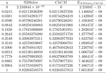
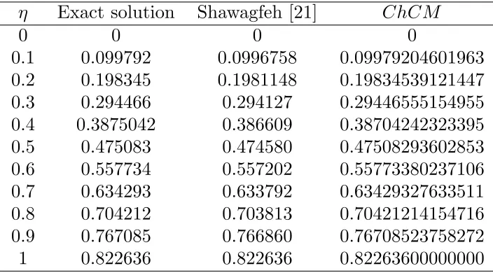
In this section, the numerical results obtained by using Chebyshev collocation method for the present physical models shall be validated through comparisons with the available exact or approximate solutions. Such comparisons are reported in terms of tables and graphs.

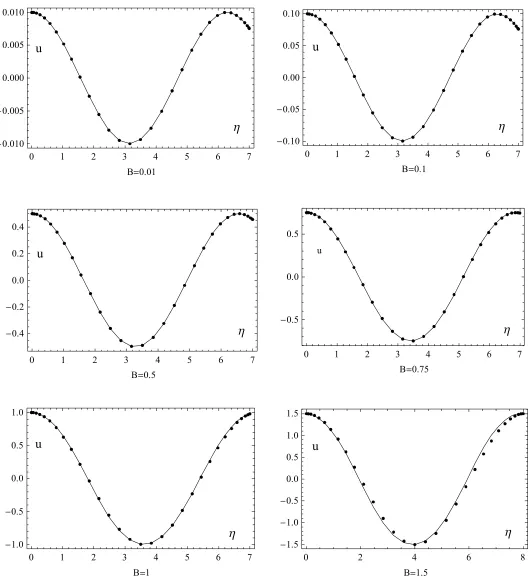
The present numerical results have been compared with the approximate solution given by Eq. (3) , where good agreement has been achieved in most cases as displayed in Fig. 1. In addition, the approximate solution given in (7) for the relativistic oscillator has been also compared with the current results in Fig. 2 and in this case the current numerical results can viewed as effective.

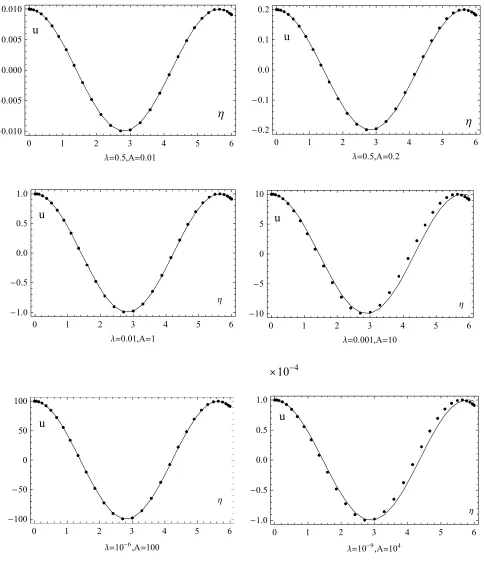
Regarding the initial value problem describing the generalized oscillator, the solution given by Eq.(11)is depicted in Fig. 3 with theChCMsolution at (Ω=ω2= 5₄, p=1,µ=−1,σ= 0,q=3)with different values forλ andA. It can be concluded form this figure that when the amplitudeAtakes high values,λ should be very small to ensure the accuracy.

obtained by Shawagfeh [21] and the the exact solution in equation (15)atm=3 as shown in Table (2₋c). These comparisons declare that the present numerical method is accurate and effective.

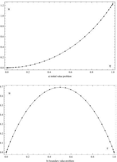
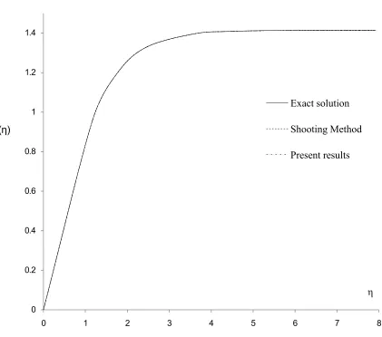
For the fifth model, the obtained numerical results have been compared with initial and boundary value problems of Bratue-type which have been discussed by Wazwaz [23] as shown in Fig. 5 (a₋b). Finally, for the sixth model 6 Table (3₋a)and Fig. 6 represent comparisons of the values of f(η) for the exact solution, the shooting method and the present method(ChCM). The maximum absolute error of Shootting method (Ee,Shooting) and (the error Ee,ChCM) of the

present method is given in Table (3₋b). From the obtained results for these fifth and sixth models we can also conclude that the current approach is accurate and therefore it can be used to analyze similar physical models.

5. Conclusion

A comprehensive numerical study is conducted for a class of nonlinear initial and boundary value problems. The results are reported in terms of tables and graphs. This is done in order to illustrate special features of the solutions. So, the obtained results using the present method indicate that it is an adequate scheme for the solution of the present problems. Therefore, the current approach may be useful to analyze similar nonlinear problems.

Conflict of Interests



u

0 1 2 3 4 5 6

0.010

0.005 0.000 0.005 0.010

a10,bc1,A0.01





u

0 1 2 3 4 5 6

0.10

0.05 0.00 0.05 0.10

a10,bc1,A0.1

u



0.0 0.5 1.0 1.5 2.0

1.0

0.5 0.0 0.5 1.0

a10,bc1,A1



u



0 1 2 3 4

1.0

0.5 0.0 0.5 1.0

a0.1,bc1,A1

u



0.0 0.5 1.0 1.5 2.0

1.0

0.5 0.0 0.5 1.0

b10,ac1,A1



u



0 1 2 3 4

1.0

0.5 0.0 0.5 1.0

c0.1,ab1,A1



u

0 1 2 3 4 5 6 7

0.010

0.005 0.000 0.005

B0.01



u

0 1 2 3 4 5 6 7

0.10

0.05 0.00 0.05

B0.1



u

0 1 2 3 4 5 6 7

0.4

0.2 0.0 0.2 0.4

B0.5



u

0 1 2 3 4 5 6 7

0.5 0.0 0.5

B0.75



u

0 1 2 3 4 5 6 7

1.0

0.5 0.0 0.5 1.0

B1



u

0 2 4 6 8

1.5 1.0 0.5 0.0 0.5 1.0 1.5

B1.5



u

0 1 2 3 4 5 6

0.010

0.005 0.000 0.005 0.010

0.5,A0.01



u

0 1 2 3 4 5 6

0.2

0.1 0.0 0.1 0.2

0.5,A0.2

 u

0 1 2 3 4 5 6

1.0

0.5 0.0 0.5 1.0

0.01,A1

 u

0 1 2 3 4 5 6

10

5 0 5 10

0.001,A10

104

 u

0 1 2 3 4 5 6

100

50 0 50 100

106,A100

 u

0 1 2 3 4 5 6

1.0

0.5 0.0 0.5 1.0

109,A104

Fig. 3. Comparison of the present results with the approximate solutionA. Ebaid15at   5

0.4 0.6

Present results

Exact u

0 0.2

0 0.2 0.4 0.6 0.8 1

Φ3

Φ2

Φ1

η



u

0.0 0.2 0.4 0.6 0.8 1.0

0.0 0.2 0.4 0.6 0.8 1.0 1.2

ainitial value problem

 u

0.0 0.2 0.4 0.6 0.8 1.0

0.0 0.1 0.2 0.3 0.4 0.5 0.6 0.7

bboundary value problem

Fig. 5ab. Comparison of the present results with intial and boundary value problem of the Bratuetype23: dots : the exact solution of intial and boundary of

0.6 0.8 1 1.2

Exact solution

Shooting Method

Present results

f(η)

0 0.2 0.4 0.6

0 1 2 3 4 5 6 7 8

Table 1. Values of

u

(

η

) for the exact solution, the Adomian decomposition

method (ADM) [22] and the present method (

ChCM

) at

m

= 3

.

η

Exact solution

Ebaid [22]

Present results

0

0

0

0

0

.

0215

0

.

021527753184314

0

.

021496840449489

0

.

021527753184314

0

.

0381

0

.

038048750666070

0

.

037994258467514

0

.

038048750666070

0

.

0590

0

.

058996522078775

0

.

058912488704097

0

.

058996522078775

0

.

0843

0

.

084140701923113

0

.

084022009055905

0

.

084140701923113

0

.

1135

0

.

113190917768906

0

.

113033703017937

0

.

113190917768906

0

.

2643

0

.

260503473299994

0

.

260193408528946

0

.

260503473299994

0

.

3087

0

.

302636337275760

0

.

302300382303633

0

.

302636337275760

0

.

4025

0

.

389261774816383

0

.

388902811746843

0

.

389261774816383

0

.

5000

0

.

475082936028531

0

.

474741879621621

0

.

475082936028531

0

.

6913

0

.

627920287048594

0

.

627693211433239

0

.

627920287048594

0

.

7357

0

.

660039308172239

0

.

659845026792322

0

.

660039308172239

0

.

8865

0

.

759023161243265

0

.

758940502736828

0

.

759023161243265

0

.

9157

0

.

776316925238970

0

.

776255547519948

0

.

776316925238970

and the present method (

ChCM

) at

m

= 2

.

η

NDSolve

ChCM

EN DSolve,ChCM

0

2

.

216844

_×

10

₀

₂

_.

₂₁₆₈

_E

₋

₂₁

0

.

0215

0

.

02112836209

0

.

02112837356

1

.

14668

E

₋

08

0

.

0381

0

.

03734293177

0

.

03734294319

1

.

14200

E

₋

08

0

.

0590

0

.

05790246281

0

.

05790246281

1

.

10838

E

₋

08

0

.

0843

0

.

08258160883

0

.

08258161968

1

.

08447

E

₋

08

0

.

1828

0

.

17821000669

0

.

17821001951

1

.

28265

E

−

08

0

.

2643

0

.

25583270380

0

.

25583271758

1

.

37779

E

−

08

0

.

3549

0

.

33982975211

0

.

33982977033

1

.

82279

E

−

08

0

.

4510

0

.

42570059687

0

.

42570060781

1

.

09385

E

−

08

0

.

5000

0

.

46794941921

0

.

46794942643

7

.

22079

E

₋

09

0

.

6913

0

.

62130146059

0

.

62130146166

1

.

06673

E

₋

09

0

.

7778

0

.

68379903935

0

.

68379903789

1

.

46641

E

₋

09

0

.

8865

0

.

75579078097

0

.

75579077351

7

.

46462

E

₋

09

0

.

9904

0

.

81731628075

0

.

81731627326

7

.

48671

E

₋

09

Table 3. Represents the values of

u

(

η

) for Mathematica (NDSolve)

and the present method (

ChCM

) at

m

= 8

.

5

.

η

NDSolve

ChCM

EN DSolve,ChCM

0

₋

5

.

41969

_×

10

₀

₅

_.

₄₁₉₆₉

_E

₋

₂₁

0

.

0215

0

.

02197144187461

0

.

02197145295276

1

.

10781

E

₋

08

0

.

0381

0

.

03883294543526

0

.

03883295616852

1

.

07333

E

₋

08

0

.

0590

0

.

06021244

.

58721

0

.

06021245745128

9

.

86407

E

₋

09

0

.

0843

0

.

08587477504774

0

.

08587478403168

8

.

98394

E

₋

09

0

.

1828

0

.

18527486029162

0

.

18527486790503

7

.

61341

E

−

09

0

.

2643

0

.

26584043801347

0

.

26584044369167

5

.

6782

E

−

09

0

.

3549

0

.

35274481836500

0

.

35274481998803

1

.

62303

E

−

09

0

.

4510

0

.

44103016433725

0

.

44103015713759

7

.

19966

E

−

09

0

.

5000

0

.

48414214397530

0

.

48414213161335

1

.

23619

E

−

08

0

.

6913

0

.

63747018932352

0

.

63747015608099

3

.

32425

E

₋

08

0

.

7778

0

.

69768758507902

0

.

69768754859829

3

.

64807

E

₋

08

0

.

8865

0

.

76438852645325

0

.

76438849111688

3

.

53364

E

₋

08

0

.

9904

0

.

81816684814189

0

.

81816681635677

3

.

17851

E

₋

08

the two terms approximation(Shawagfeh) [21]

and the present method (

ChCM

) at

m

= 3

.

η

Exact solution

Shawagfeh [21]

ChCM

0

0

0

0

0

.

1

0

.

099792

0

.

0996758

0

.

09979204601963

0

.

2

0

.

198345

0

.

1981148

0

.

19834539121447

0

.

3

0

.

294466

0

.

294127

0

.

29446555154955

0

.

4

0

.

3875042

0

.

386609

0

.

38704242323395

0

.

5

0

.

475083

0

.

474580

0

.

47508293602853

0

.

6

0

.

557734

0

.

557202

0

.

55773380237106

0

.

7

0

.

634293

0

.

633792

0

.

63429327633511

0

.

8

0

.

704212

0

.

703813

0

.

70421214154716

0

.

9

0

.

767085

0

.

766860

0

.

76708523758272

Table 5. Values of

f

(

η

) for the exact solution, the shooting method and

the present method (

ChCM

)

.

η

The exact solution

ChCM

Shootting method

0

0

0

3

.

1102

_×

10

1

.

17157

0

.

961141183786619

0

.

9611070045979400

0

.

9611054342686112

1

.

77772

1

.

202428601606520

1

.

2023643183102284

1

.

2023645509982483

2

.

46927

1

.

330665896574968

1

.

3305704365379722

1

.

330570838696424

3

.

60793

1

.

397114413277153

1

.

3969685880488372

1

.

396968522682298

4

.

39207

1

.

4085494708083601

1

.

4083673080884052

1

.

408367284942106

5

.

16114

1

.

4123021434700513

1

.

4120834942495526

1

.

4120834612222437

5

.

88559

1

.

4135271302075076

1

.

4132736020214456

1

.

4132735693434024

6

.

53757

1

.

4139405233760458

1

.

4136553770920586

1

.

4136553408479557

7

.

09204

1

.

4140889100927603

1

.

4137767754240098

1

.

4137767398762842

7

.

52769

1

.

4141462431225706

1

.

4138128682103317

1

.

4138128330749593

7

.

92314

1

.

4141750797928212

1

.

4138224084323320

1

.

4138223729952500

E

E

0

3

.

1102

_×

10

618 NADER Y. ABD ELAZEM, ABDELHALIM EBAID REFERENCES

[1] Fox L and Parker I B, 1968, Chebyshev polynomials in numerical analysis, Clarendon Press Oxford. [2] Gottlieb D and Orszag S A 1977 Numerical analysis of spectral methods: theory and applications, in:

CBMS-NSF Regional Conference series Applied Mathematics vol. 26 SIAM Philadelphia PA

[3] Canuto C, Hussaini M Y and Zang T A 1988. Spectral Methods in Fluid Dynamics Springer-Verlag New York

[4] Voligt, R G, Gottlieb D and Hussaini M Y 1984 Spectral methods for partial differential equations SIAM Philadelphia PA

[5] Boyd J P 1989 Chebyshev and Fourier Spectral Methods Springer-Verlag New York

[6] Kidder L E, Scheel M A, Teukolsky S A, Carlson E D, and Cook G B 2000 Black hole evolution by spectral methods Phys. Rev. D 62 1–20

[7] Peyret R 2002 Spectral Methods for Incompressible Viscous Flow Springer-Verlag New York [8] Snyder M A 1966 Chebyshev Methods in Numerical Approximation Prentice-Hall USA

[9] Yang H H, Seymour B R and Shizgal B D 1994 A Chebyshev pseudospectral multi-domain method for steady flow past a cylinder, up to Re = 150 Comput. Fluids 23 829–851

[10] Boyd J P 2000 Chebyshev and Fourier Spectral Methods Dover New York

[11] Elbarbary E M E 2005 Chebyshev finite difference method for the solution of boundary-layer equations Appl. Math. Comput. 160 487–498

[12] Elbarbary E M E and El-Kady M 2003 Chebyshev finite difference approximation for the boundary value problems Appl. Math. Comput. 139 513–523

[13] Elbarbary E M E and El-Sayed S M 2005 Higher order pseudospectral differentiation matrices Appl. Numer. Math. 55 425–438

[14] Hua Chen Guo, Ling Tao Zhao and Zhong Min Jin 2011 Notes on a conservative nonlinear oscillator Com-puters Math. Applic. 61 2120-2122

[15] Ebaid Abdelhalim 2010 Analytical periodic solution to a generalized nonlinear oscillator: application of He’s frequency-amplitude formulation Mechanics Research Communications 37 111–112

[16] Chu Cai Xu and Ying Wu Wen 2009 He’s frequency formulation for the relativistic harmonic oscillator Computers Math. Applic. 58 2358-2359

[17] Fan Jie 2009 He’s frequency–amplitude formulation for the Duffing harmonic oscillator Computers Math. Applic. 58 2473-2476

[18] Fang Liu Jun 2009 He’s variational approach for nonlinear oscillators with high nonlinearity Computers Math. Applic. 58 2423-2426

[20] Li Zhang Lui 2009 Periodic solutions for some strongly nonlinear oscillations by He’s energy balance method Computers Math. Applic. 58 2480-2485

[21] Shawagfeh N T 1996 Analytic approximate solution for a nonlinear oscillator equation Computers Math. Applic. 31 6 135-141

[22] Ebaid Abdelhalim 2010 Modification of Lesnic’s Approach and New Analytic Solutions for Some Nonlinear Second-Order Boundary Value Problems with Dirichlet Boundary Conditions Z. Naturforsch. 65a 692 – 696 [23] Wazwaz Abdul- Majid 2005 Adomian decomposition method for a reliable treatment of the Bratu-type

equa-tions Applied Mathematics and Computation 166 652–663

[24] Zhou Yongfang, Lin Yinzhen and Cui Minggen 2007 An efficient computational method for second order boundary value problems of nonlinear differential equations Applied Mathematics and Computation 194 354–365

[25] Elgazery N S and Abd Elazem N Y 2008 Chebyshev collocation method for the effect of variable thermal conductivity on micropolar fluid flow over vertical cylinder with variable surface temperature Journal of Applications and Applied Mathematics 3 2 286-307

[26] Elgazery N S and Abd Elazem N Y 2009 Effects of variable properties on MHD unsteady mixed-convection in non-Newtonian fluid with variable surface temperature Journal of Porous Media 12 5 477-488.

[27] Elgazery N S and Abd Elazem N Y 2009 The effects of variable properties on MHD unsteady natural con-vection heat and mass transfer over a vertical wavy surface International Journal of Mechanica 44 573-586 [28] Elgazery N S and Abd Elazem N Y 2010 Chebyshev collocation method for the effect of variable thermal

conductivity on micropolar fluid flow Journal of Chemical Engineering Communications 197 3 400 - 422 [29] Elgazery N S and Abd Elazem N Y 2011 Effects of viscous dissipation and Joule heating on natural

convec-tion flow of a viscous fluid from heated vertical wavy surface Journal of Zeitschrift f¨ur Naturforschung A – Physical Sciences 66a 2011 427-440

[30] Abd Elazem N Y and Ebaid A 2011 Comparison of numerical methods for nano boundary layer flow Z. Naturforsch. 66a 539 – 542

[31] Buckmire R 2003 Investigations of nonstandard Mickens-type finite-difference schemes for singular bound-ary value problems in cylindrical or spherical coordinates Numerical Methods for partial Differential equa-tions 19 3 380–398

[32] Aregbesola Y 2003 Numerical solution of Bratu problem using the method of weighted residual Electronic Journal of Southern African Mathematical Sciences Association 3 01 1–7