DEMOGRAPHIC RESEARCH
A peer-reviewed, open-access journal of population sciences
DEMOGRAPHIC RESEARCH
VOLUME 31, ARTICLE 22, PAGES 659–688
PUBLISHED 17 SEPTEMBER 2014
http://www.demographic-research.org/Volumes/Vol31/22/ DOI: 10.4054/DemRes.2018.31.22
Research Article
Unobserved population heterogeneity:
A review of formal relationships
James W. Vaupel
Trifon I. Missov
c
2018 James W. Vaupel & Trifon I. Missov.
1 Population heterogeneity 660
2 Notation and terminology 660
3 General results 662
4 Relationships for relative-risk models with fixed frailty 665 5 Relationships for relative-risk models with gamma-distributed fixed frailty 669 6 Relationships for relative-risk models with gamma-distributed fixed frailty and Gompertz
haz-ard (gamma-Gompertz (ΓG) models) 674
7 Relationships for relative-risk models with gamma-distributed fixed frailty and Gompertz-Makeham hazard (gamma-Gompertz-Gompertz-Makeham (ΓGM) models) 678
8 Conclusion 680
9 Acknowledgments 681
References 682
Unobserved population heterogeneity:
A review of formal relationships
James W. Vaupel1
Trifon I. Missov2
Abstract
BACKGROUND
Survival models accounting for unobserved heterogeneity (frailty models) play an impor-tant role in mortality research, yet there is no article that concisely summarizes useful relationships.
OBJECTIVE
We present a list of important mathematical relationships that govern populations in which individuals differ from each other in unobserved ways. For some relationships we present proofs that, albeit formal, tend to be simple and intuitive.
METHODS
We organize the article in a progression, starting with general relationships and then turn-ing to models with stronger and stronger assumptions.
RESULTS
We start with the general case, in which we do not assume any structure of the underlying baseline hazard, the frailty distribution, or their link to one another. Then we sequentially assume, first, a relative-risk model; second, a gamma distribution for frailty; and, finally, a Gompertz and Gompertz-Makeham specification for baseline mortality.
COMMENTS
The article might serve as a handy overall reference to frailty models, especially for mor-tality research.
1Max Planck Institute for Demographic Research, Rostock, Germany. Max-Planck Odense Center on the
Biodemography of Aging, University of Southern Denmark, Odense, Denmark. Duke University Population Research Institute, Durham, NC 27705 USA
2Max Planck Institute for Demographic Research, Rostock, Germany. University of Rostock, Institute of
1. Population heterogeneity
Unobserved heterogeneity plays an important role in shaping mortality trajectories for populations. An overview of unobserved heterogeneity in demographic research can be found in Yashin, Iachine, and Begun (2000) and Vaupel and Yashin (2001b,a, 2006). Vau-pel and Yashin (1985) present a number of examples in which hazards of individuals or subpopulations and the hazard of the entire population follow different trajectories. We do not review that material here and we do not discuss applications to the analysis of empirical data; the aim of this article is to present the key mathematical relationships that hold in models with unobserved heterogeneity. We start with the general case and intro-duce increasingly restrictive assumptions about the distributions of baseline mortality and unobserved heterogeneity (see Figure 1). We present short proofs and derivations as well as some brief qualitative interpretations.
Figure 1: Structure of the presentation of relationships
General Setting
Relative Risks and Fixed Frailty
Gamma Frailty
Gompertz Hazard
Gompertz-Makeham Hazard
2. Notation and terminology
In frailty models we distinguish between the mortality schedules for individuals and the entire population. The model for individuals depends on a random variableZ, called
frailty(Vaupel, Manton, and Stallard 1979), that is unobserved. As a result individual mortality is captured by a conditional (on frailty) distribution. For a given realizationz of frailtyZwe denote theforce of mortality(also known as theintensity of mortality, the
s(x, z) = exp
−
x Z
0
µ(t, z)dt
and µ(x, z) =−dlns(x, z)
dx . (1)
We assume that the distribution of frailty among survivors to agexis characterized by a probability density function (p.d.f.) π(x, z). The p.d.f. of frailty at the starting age of analysis isπ(0, z).
The hazard for the population
¯ µ(x) =
∞
Z
0
µ(x, z)π(x, z)dz (2)
and the survival function for the population
¯ s(x) =
∞
Z
0
s(x, z)π(0, z)dz (3)
are often designated byµ(x)ands(x), but we prefer the version with a bar-sign on top as these functions are “averages” with respect to the frailty distribution. We will refer to (2) and (3) as thepopulation,marginal, oraggregate (population) hazard/survival function
and use these terms interchangeably. They are linked to one another by relationships that are analogical to (1).
We designate the age-derivative and the relative age-derivative of a function by a dot and an accent, respectively; e.g., forµ¯(x)we denote
˙¯
µ(x) = d
dxµ¯(x) and µ´¯(x) =
d dxµ¯(x)
¯
µ(x) . (4)
This notation is not new; it can be traced back to Vaupel, Manton, and Stallard (1979) and Vaupel (1992). Many important demographic relationships have been expressed in such notation (see, e.g., Vaupel and Canudas-Romo 2003; Vaupel and Zhang 2010). Table A.1 summarizes the basic notation and terminology we use in the following sections.
so easy that we did not feel that a formal proof was necessary. Again if readers disagree, we will provide additional proofs in future versions of the Primer. One of the advantages of publishing in Demographic Research is that articles can be revised as appropriate.
3. General results
General Setting
Relative Risks and Fixed Frailty
Gamma Frailty
Gompertz Hazard
Gompertz-Makeham Hazard
Suppose, in a population, individuals are characterized byZ, a random variable ac-counting for unobserved heterogeneity, with p.d.f. π(0, z)at a given starting age. We will useZto denote a random variable andzto denote a particular value of this random variable for an individual. Suppose the individuals die or otherwise exit according to a schedule specified by hazardµ(x, z)and survival function s(x, z). Then the following relationships hold:
3A. Cohort survivorship in a populations¯(x)is the weighted average of conditional sur-vival functionss(x, z)that correspond to all profilesπ(0, z)in the study population:
¯ s(x) =
∞
Z
0
π(0, z)s(x, z)dz . (5)
If the population is stratified into a countable number of subgroups, i.e. whenπ(0, z) is discrete, (5) becomes
¯
s(x) =X
z
π(0, z)s(x, z), (6)
3B. The density of the frailty distribution among survivors to agexis given by
π(x, z) =π(0, z)s(x, z) ¯
s(x) . (7)
This can be rewritten as
s(x, z) =π(x, z)
π(0, z)s¯(x), (8) a formula, due to Vaupel (1992), used in “fixed attribute dynamics” to study, e.g., the survival of persons with some genotype based on data on the prevalence of the genotype at two successive ages (Gerdes et al. 2000; Zeng and Vaupel 2004).
3C. Ife(0, z)denotes life expectancy at birth for the subpopulation withZ=z, then life expectancy at birth for the entire population¯e(0)is a weighted average ofe(0, z) across all profiles (Vaupel 1988):
¯ e(0) =
∞
Z
0
e(0, z)π(0, z)dz . (9)
3D. The population hazardµ¯(x)is the weighted average of the hazardsµ(x, z)of all subpopulations at agex, weighted by the distributionπ(x, z)atx:
¯ µ(x) =
∞
Z
0
µ(x, z)π(x, z)dz . (10)
It is the negative relative derivative of the population survivorships¯(x):
¯
µ(x) =−
d dxs¯(x)
¯
s(x) =−´¯s(x). (11)
3E. An identical relationship holds for remaining life expectancy¯e(x)at agex– only those individuals that survived toxcount (Vaupel 1988):
¯ e(x) =
∞
Z
0
3F. The derivative of the population hazard can be expressed as (Vaupel 1992; Vaupel and Zhang 2010)
˙¯
µ(x) = ¯˙µ(x)−σ2µ(x), (13) where
˙¯
µ(x) = d
dxµ¯(x) = d dx
∞
Z
0
µ(x, z)π(x, z)dz ,
is the change in the hazard for the entire population at agex,
¯˙ µ(x) =
∞
Z
0
d
dxµ(x, z)π(x, z)dz
is the average change in all individual hazardsµ(x, z)atx, and
σµ2(x) =
∞
Z
0
µ2(x, z)π(x, z)dz−µ¯2(x)
is the variance of µ(x, z)across all profiles. Eq. 13 implies that individuals age faster than populations:µ¯˙(x)>µ˙¯(x).
Proof. This is a special case of the more general relationship for derivatives of av-erages (see Price 1970; Vaupel 1992; Vaupel and Canudas-Romo 2003). The proof follows from simple differentiation of
¯ µ(x) =
∞
R
0
µ(x, z)s(x, z)π(0, z)dz
∞
R
0
s(x, z)π(0, z)dz
by expressing dxd s(x, z) =−µ(x, z)s(x, z).
3G. The difference between the values of the population hazard at two different ages can be usefully decomposed in the following way:
¯
µ(x2)−µ¯(x1) = [ ¯µ(x2)−µ˜(x1) ] + [ ˜µ(x1)−µ¯(x1) ] (14) ∀x2 > x1 ≥ 0, whereµ˜(x1)is the population hazard at agex1 of survivors to
population hazard among survivors tox2, and the second term measures the change
in the composition of the population due to differential survival. Relationship (14) was introduced by Rebke et al. (2010) for any average characteristic of a population.
4. Relationships for relative-risk models with fixed frailty
General Setting
Relative Risks and Fixed Frailty
Gamma Frailty
Gompertz Hazard
Gompertz-Makeham Hazard
The results presented above hold for any population in which the value ofZfor an indi-vidual is independent of the value ofZfor any other individual. The indexzcould pertain to a fixed number (realization of a random variable) or vector of numbers (realization of a random vector). Indeed, an individual might have a vectorz= (z1, z2, . . .)that uniquely
defines a stochastic mortality or attrition trajectory. In this section we restrict ourselves to a fixed single frailty parameter that acts multiplicatively on the baseline hazard. We do not specify, though, any parametric distribution for it. In a multiplicative (proportional-hazard, relative-risk) fixed-frailty model (Vaupel et al. 1979), Z can be interpreted as “frailty”, and the individual force of mortality is defined as
µ(x, z) =z µ(x), (15)
whereµ(x)≡µ(x,1)is the baseline hazard. In this setting, the following relationships hold:
4A. The population hazardµ¯(x)at any agexis a function of the baseline hazardµ(x) and the average frailtyz¯(x) =
∞
R
0
z π(x, z)dzamong survivors to this age (Vaupel, Manton, and Stallard 1979)
¯
Because frailer individuals die out first,¯z(x)decreases with agexand, as a result, the force of mortality for individuals increases faster than the force of mortality for the population as a whole.
4B. A similar relationship links the changes in the hazards of individuals and the popu-lation:
¯˙
µ(x) = ¯z(x) ˙µ(x). (17*) Asz¯(x)declines, the change in the force of mortality for the population becomes smaller than the change in the baseline hazard.
Proof.
¯˙ µ(x) =
∞
Z
0
˙
µ(x)z π(x, z)dz= ¯z(x) ˙µ(x)
4C. The variance of the conditional hazard at agexequals the product of the squared baseline hazard and the variance of the frailty distribution atx
σµ2(x) =µ2(x)σz2(x), (18*)
whereσz2(x) =
∞
R
0
z2π(x, z)dz−z¯2(x).
Proof.
σµ2(x) =
∞
Z
0
z2µ2(x)π(x, z)dz−
∞
Z
0
z µ(x)π(x, z)dz
2
=
= µ2(x)
∞ Z 0
z2π(x, z)dz−
∞
Z
0
z π(x, z)dz
2 =
= µ2(x)σz2(x)
A simple corollary is that the squared coefficients of variation of conditional mortal-ity and frailty are equivalent at any agex:
Proof.
CV2µ(x) = σ
2
µ(x)
¯ µ2(x) =
µ2(x)σz2(x) ¯
z2(x)µ2(x) =CV 2
z(x)
4D. The relative derivative of the population hazard can be expressed as
´ ¯
µ(x) = ´µ(x)−µ¯(x)CV2z(x). (20*)
Proof. Divide both sides of (13) byµ¯(x)and take advantage of (17*) and (19*).
Eq. 20* has a useful implication (Missov and Vaupel 2014). Suppose the population hazard levels off after agex∗, i.e.
¯
µ(x) = ¯µ∗≡const ∀x≥x∗>0. (21) Then the (relative) derivative of the population hazard vanishes
˙¯
µ(x) = ´µ¯(x) = 0 (22)
and (20*) is reduced to
´
µ(x) = ¯µ∗·CV2z(x). (23) Although this equation has infinitely many solutions, two special cases offer straight-forward demographic interpretation:
1. µ´(x) = CV2z(x) = 0, which implies a homogeneous population exposed to a constant hazard, and
2. µ´(x) =b≡constand CV2z(x) =γ ≡const, which implies a Gompertz base-line and gamma-distributed frailty (Missov 2012; Missov and Vaupel 2014).
4E. The average frailty of the dead atx
z†(x) =
∞
R
0
z µ(x, z)π(x, z)dz
∞
R
0
µ(x, z)π(x, z)dz
(24)
can be expressed (Vaupel, Manton, and Stallard 1979) as
z†(x) = ¯z(x)
1 +CV2z(x)
Proof. Follows by substituting (15) under the integrals in (24) and reorganizing terms.
The major analytical advantage of assuming relative risks is that the marginal distri-bution can be expressed from the conditional distridistri-bution through the Laplace trans-form (Laplace 1782, 1785), the properties of which have been thoroughly studied by Doetsch (1937, 1950, 1955, 1956). The Laplace transform of a functionf(z)is defined as
L(s) =
∞
Z
0
e−szf(z)dz . (26)
If f(z)is a p.d.f. of a random variableZ, then (26) is the expected value of the random variablee−sZ. In this case the Laplace transform is also denoted byL
Zand
is called theLaplace transform ofZor theLaplace transform of the distribution ofZ.
4F. Population survival at agexis the Laplace transform of the frailty distribution cal-culated at the baseline cumulative hazard
¯
s(x) =LZ(H(x)), (27)
whereLZ(·)is the Laplace transform of the frailty distribution at the initial age and
H(x) =Rx
0 µ(x)dxis the baseline cumulative hazard. The hazard of the population
¯
µ(x)can be then expressed via the same Laplace transform and the baseline hazard:
¯
µ(x) =−µ(x) d
dslnLZ(s)
s=H(x)
=−µ(x) ´LZ(s)
s=H(x) . (28)
Proof. The expression fors¯(x)follows by expressings(x, z)in terms ofH(x, z) = zH(x)
¯ s(x) =
∞
Z
0
s(x, z)π(0, z)dz=
∞
Z
0
e−zH(x)π(0, z)dz=LZ(H(x))
5. Relationships for relative-risk models with gamma-distributed
fixed frailty
General Setting
Relative Risks and Fixed Frailty
Gamma Frailty
Gompertz Hazard
Gompertz-Makeham Hazard
All results in the previous section hold when frailty acts multiplicatively on the baseline hazard. In this section we will make the additional assumption that frailty is gamma-distributed (Vaupel, Manton, and Stallard 1979). The gamma distributionΓ(k, λ)with positive parametersk, λhas a density
π(0, z) = λ
k
Γ(k)z
k−1e−λz. (29)
Frailty is often assumed to be gamma-distributed for several reasons. First, the gamma distribution has a flexible shape and converges to a normal distribution ask → ∞ (di-rect corollary of the central limit theorem). Second, the gamma distribution has a simple Laplace transform(1 +s/λ)−k(Mellin 1900), which makes working with the marginal distribution convenient. Third,π(x, z)is gamma distributed at all agesxwith the samek andλ(x) =λ+H(x). Finally, the gamma distribution has a regularly varying density, which is the property frailty distributions possess in a wide family of survival models with unobserved heterogeneity (Missov and Finkelstein 2011). Ifπ(0, z)is a regularly varying density, thenπ(x, z)will approach a gamma distribution ass¯(x)approaches zero (see Abbring and van den Berg 2007; Missov and Finkelstein 2011; Missov and Vaupel 2014). In relative-risk models with gamma-distributed fixed frailty, the following rela-tionships hold:
5A. 1. The average frailty of survivors to agexor, formally speaking, the expected value of the frailty random variable at age x, equals (Vaupel, Manton, and Stallard 1979)
¯
z(x) = k
Proof. Using (7) ands(x, z) = [s(x)]z=e−zH(x), we get
¯ z(x) =
∞
Z
0
z π(x, z)dz= 1 ¯ s(x)
∞
Z
0
z π(0, z)s(x, z)dz=
=
1 +H(x) λ
k kλk
(λ+H(x))k+1 = k λ+H(x).
2. Suppose the frailty distribution at the starting age has a unit expectationz¯(0) = 1. This means that the “average” or “standard” individual is subjected to the baseline hazardµ(x). A mean of one impliesk=λ= 1/γ, whereγcan be interpreted as the squared coefficient of variation ofZat any agex. Then (Vaupel, Manton, and Stallard 1979)
¯
z(x) = 1
1 +γ H(x). (31)
Proof. Follows directly from (30).
5B. 1. Vaupel, Manton, and Stallard (1979) showed that population survival in a relative-risk model with fixed gamma-distributed frailty is given by
¯
s(x) =LZ(H(x)) =
1 +H(x) λ
−k
. (32)
In addition, ifz¯(0) = 1, then
2.
¯
s(x) = (1 +γH(x))−1γ (33)
and
3.
¯
z(x) = [¯s(x)]γ. (34)
5C. Ifz¯(0) = 1, then (Vaupel 2002)
1.
¯
µ(x) =µ(x) [¯s(x)]γ (35)
and (Vaupel, Manton, and Stallard 1979)
2.
¯
µ(x) = µ(x)
1 +γH(x). (36) 5D. In a relative-risk model with fixed gamma-distributed frailty the average frailty of
the dead can be expressed as (Vaupel, Manton, and Stallard 1979)
¯
z†(x) = ¯z(x)·(1 +γ). (37)
Proof. Follows directly from (25) taking into account that the squared coefficient of variation for gamma-distributed frailty at any agexis equal toγ.
5E. Suppose the baseline hazardsµ1(x)andµ2(x)of two populations are proportional
by a factor ofR:
µ2(x) =R µ1(x), (38)
where, without loss of generality,R >1. Then
1. if frailty is gamma-distributed with mean 1 and squared coefficient of variationγ forbothpopulations, the marginal hazardsµ¯1(x)andµ¯2(x)of the two
popula-tions converge (Manton and Stallard 1981).
Proof. Eq. 38 implies thatH2(x) =R H1(x). Using in addition (16) and (31),
we get
¯
R(x) := µ¯2(x) ¯ µ1(x)
=R+R γH1(x) 1 +R γH1(x)
.
¯
R(x)>1becauseR >1and lim
x→∞
¯
R(x) = 1.
2. if frailty is gamma distributed with mean 1 for both populations, but the respective squared coefficients of variationγ1andγ2are such thatγ2 > γ1, then there is a
Proof. On the one hand,
¯
R(0) =R >1.
and, on the other hand,
lim
x→∞
¯
R(x) = lim
x→∞
R+R γ1H1(x)
1 +R γ2H1(x)
= γ1 γ2
<1.
Hence there is a crossover atx0, at whichH1(x0) = R(γR2−−1γ1).3
5F. Suppose there exists an agex∗such that
µ2(x) =
R µ1(x), x < x∗
R∗µ1(x), x≥x∗,
whereR > 1andR∗are constants, and frailty is gamma-distributed with mean 1 and squared coefficient of variationγforbothpopulations. Then there is a crossover ofµ¯1(x)andµ¯2(x)ifR∗<1+R γH1(x
∗)
1+γH1(x∗) . Proof. Forx < x∗
¯
R(x) = R+R γH1(x) 1 +R γH1(x)
>1.
Atx=x∗
¯
R(x∗) = R
∗[1 +γH
1(x∗)]
1 +R γH1(x∗)
.
This quantity is less than 1 (i.e., there is a crossover) if
R∗<1 +R γH1(x
∗)
1 +γH1(x∗)
.
Note thatR∗can exceed 1.4
5G. Demographic models have often two time dimensions (age and period) with a third one (cohort) being their linear combination. As a result survival models in demog-raphy are often defined on a surface. The negative relative derivative ofµ¯(x, y)with respect to yearyis denoted asρ¯(x, y)and captures yearly mortality improvement:
¯
ρ(x, y) =− 1
¯ µ(x, y)
∂
∂yµ¯(x, y).
In a relative-risk model with gamma-distributed frailtyρ¯(x, y)can be expressed as
¯
ρ(x, y) =ρ(x, y)−γ´¯sc(x, y) (39*)
where¯sc(x, y)denotes survival to agexfor the cohort born iny−x,
´ ¯
sc(x, y) =−
1 ¯ sc(x, y)
∂
∂ys¯c(x, y), and
ρ(x, y) =− 1
µ(x, y) ∂
∂yµ(x, y).
Hence the rate of progress for the population is less than the rate of progress for the individuals in the population.
Proof. By analogy to the uni-dimensional case (35), we have ¯
µ(x, y) =µ(x, y) ¯sγc(x, y).
Combining the latter with the definitions ofρ¯(x, y)andρ(x, y), we get
¯
ρ(x, y) =−
∂
∂yµ(x, y)·¯s γ
c(x, y) +µ(x, y)· ∂ ∂ys¯
γ c(x, y)
µ(x, y) ¯sγc(x, y)
=
=ρ(x, y)−
∂ ∂y¯s
γ c(x, y)
¯
sγc(x, y) =
ρ(x, y)−γ
∂
∂ys¯c(x, y)
¯ sc(x, y)
6. Relationships for relative-risk models with gamma-distributed
fixed frailty and Gompertz hazard (gamma-Gompertz (ΓG)
models)
General Setting
Relative Risks and Fixed Frailty
Gamma Frailty
Gompertz Hazard
Gompertz-Makeham Hazard
A further level of detail in survival models with unobserved heterogeneity can be reached by specifying the baseline distribution. For various theoretical and empirical reasons the Gompertz exponential-increase law (Gompertz 1825) is often assumed as the baseline hazard in models of adult mortality. The Gompertz function can be expressed as
µ(x) =aebx=beb(x−M),
wherea =µ(0)is the hazard at the initial age,b is the rate of increase, andM is the mode (Missov et al. 2014).
In aΓG model withk=λ= 1/γthe following relationships hold:
6A. The population hazard can be represented in several equivalent forms:
1. in terms of the ΓG parameters only (Vaupel, Manton, and Stallard 1979; Missov et al. 2014)
¯
µ(x) = ae
bx
1 + aγ b (e
bx−1) =
beb(x−M)
1 +γe−bM(ebx−1). (40)
Proof. Follows from (36) taking into account the functional form of the Gom-pertz baseline cumulative hazard
H(x) =a b(e
bx−1) =e−bM(ebx−1). (41)
2. in terms of the baseline hazard, the observed cohort survivorship¯s(x)from the initial age to agex, and the squared coefficient of variation γ of frailty (Vaupel 2002)
¯
µ(x) =aebx[¯s(x)]γ =beb(x−M)[¯s(x)]γ . (42)
Proof. Follows from (35) taking into account the expression for the Gompertz hazardµ(x) =aebx=beb(x−M).
3. incorporating information about the mortality plateau
¯
µ(x) ={1−[¯s(x)]γ}µ¯∗+ [¯s(x)]γµ¯0, (43*)
whereµ¯∗ = lim
x→∞µ¯(x) =b/γdenotes the plateau andµ¯0 = ¯µ(0) =ais the
mortality level at the starting age.
Proof. We expressebxfrom
¯
s(x) =1 + aγ b (e
bx−1)−
1 γ
(a corollary of (33) for a Gompertz baseline) and substitute it in (42).
1. in terms of theΓG parameters only (Vaupel, Manton, and Stallard 1979)
¯
z(x) =h1 +aγ b (e
bx−1)i−1. (44)
Proof. Follows from (31) and (41).
2. incorporating information about the mortality plateau
¯ z(x) =µ¯
∗−µ¯(x)
¯ µ∗−µ¯
0
. (45*)
Proof. Follows from (43*) by taking¯z(x) = [¯s(x)]γinto account and
reorga-nizing terms.
3. rewriting (45*) in terms of parametersbandγ
¯
z(x) = b−γµ¯(x) b−γµ¯0
. (46*)
Proof. We take advantage of the fact thatµ¯∗=b/γ.
6C. Population survivorship can also be expressed in three alternative ways: 1. in terms of theΓG parameters only (Vaupel, Manton, and Stallard 1979)
¯
s(x) =h1 +aγ b (e
bx−1)i−
1 γ
. (47)
Proof. Population survivorship is the Laplace transform of the frailty distri-bution calculated for the baseline cumulative hazard. The relationship follows directly from (33) taking into account the form of the Gompertz cumulative hazard.
2. incorporating information about the mortality plateau
¯ s(x) =
µ¯∗−µ¯(x)
¯ µ∗−µ¯
0
µ¯ ∗
b
. (48*)
Proof. Follows froms¯(x) = [¯z(x)]1/γ = [¯z(x)]µ¯∗/band (45*).
3. rewriting (48*) in terms of parametersbandγ
¯ s(x) =
b−γµ¯(x)
b−γµ¯0
1γ
6D. The rate of aging¯b(x)of a population, known as LAR, the lifetable aging rate (Ho-riuchi and Coale 1990), is usually defined in demography as the relative derivative of the population force of mortalityµ¯(x)with respect to agex:
¯b(x) = 1 ¯ µ(x)
d
dxµ¯(x). (50)
In aΓG model¯b(x)can be represented in at least two different ways. In both cases the individual rate of agingbexceeds the rate of aging¯b(x)of the population.
1.
¯b(x) =b−γµ¯(x) (51*)
Proof. Taking the derivative ofµ¯(x)with respect toxleads to:
¯
b(x) =µ¯˙(x) ¯ µ(x)−
σ2
µ(x)
¯ µ(x) .
The first term on the right-hand side is equal to b for a Gompertz baseline µ(x) = aebx. The second term can be represented as a product ofµ¯(x)and the squared coefficient of variation ofµ(x, z)(or, using (19*), of frailty) at agex:
σ2
µ(x)
¯
µ(x) = ¯µ(x) σ2
µ(x)
¯
µ2(x) = ¯µ(x)CV 2
µ(x) = ¯µ(x)CV
2
z(x).
The squared coefficient of variation of the gamma distribution depends only on the shape parameter and equals1/k. As the distribution of frailty for all xis gamma with one and the same shape parameterk = 1/γ, CV2z(x) =γ,
which completes the proof.
2.
¯ b(x) =b
1−µ¯(x)
¯ µ∗
(52*)
General Setting
Relative Risks and Fixed Frailty
Gamma Frailty
Gompertz Hazard
Gompertz-Makeham Hazard
7. Relationships for relative-risk models with
gamma-distributed fixed frailty and Gompertz-Makeham
hazard (gamma-Gompertz-Makeham (ΓGM) models)
A standard extension of the Gompertz model is to add a constant term that ac-counts for extrinsic mortality, not related to aging processes (Makeham 1860). The resulting gamma-Gompertz-Makeham (ΓGM) fixed-frailty model is defined by a conditional hazard
µ(x, z) =z aebx+c ,
which fork=λ= 1/γresults in the following population hazard (Manton, Stal-lard, and Vaupel 1981)
¯
µ(x) = ae
bx
1 + aγb (ebx−1) +c . (53)
This is an additive-hazards model with a Gompertz age-dependent component af-fected by frailty, and a constant Makeham componentcaccounting for non-aging-related mortality. Most relationships derived for the gamma-Gompertz model (ad-justed forc) hold in theΓGM settting, too. The only substantial difference concerns the rate of aging¯b(x)for the population.
7A. Vaupel and Zhang (2010) present an exact expression for¯b(x)inΓGM mod-els:
¯b(x) =µ˙¯(x) ¯ µ(x)=b
1− c
¯ µ(x)
−γ
1− c
¯ µ(x)
[¯µ(x)−c]. (54)
Proof. One should take advantage of (53) and reorganize terms.
¯ b(x) =b
1− c
¯ µ(x)
¯
µ∗−µ¯(x) ¯
µ∗−c . (55)
Proof. At the plateau¯b(x) = 0andµ¯(x) = ¯µ∗, which impliesγ=b/(¯µ∗−
c). Substitutingγ in (54) and reorganizing terms accordingly completes the proof.
7C. If in additionc≈0, i.e., whenµ(x)≈aebx, then
¯b(x)≈b
1−µ¯(x)
¯ µ∗
. (56)
This is an approximate multiplicative relationship between¯b(x) = ´µ¯(x), the rate of aging for the population, andb= ´µ(x), the rate of aging for individu-als. Ifc= 0, then the exact relationship (56) holds.
7D. A widely used demographic indicator in comparative research is the remaining life expectancy at agex, denoted bye(x)and expressed as
e(x) =
∞
Z
x
t d(t)dt= 1 s(x)
∞
Z
x
s(t)dt . (57)
From a statistics perspective, this represents the first moment (i.e., mean) of the underlying distribution of deaths after agex. Life expectancy in a gamma-Gompertz-Makeham framework equals (Missov and Lenart 2013)
e(x) = (bλ)
ke−(bk+c)x
ak(bk+c) 2F1
k+c b, k;k+
c b + 1;
1−bλ
a
e−bx
,
(58) where
2F1(α, β;γ;z) =
∞
X
j=0
(α)j(β)j
(γj)
zj
j! , (59)
is the Gaussian hypergeometric function defined for γ > β > 0 (see, for example, Bailey 1935). Forn ∈ N,(m)n = m(m+ 1). . .(m+n−1)
denotes the Pochhammer symbol with(m)0 = 1. Note that forx= 0(58)
provides an expression for life expectancy at birth.
Note that forc = 0andx= 0(58) is reduced to an expression for gamma-Gompertz life expectancy (Missov 2013)
e(0) = 1 bk2F1
k,1;k+ 1; 1− a
bλ
. (60)
8. Conclusion
Unobserved heterogeneity should not be overlooked when fitting models to time-to-event data, as this might lead to dubious estimation results (Elbers and Ridder 1982; Heckman and Singer 1982). It can be captured by a random variable (frailty) that accounts for individual susceptibility. We presented a list of relationships, starting from the general setting, in which no assumptions about the baseline haz-ard or the frailty distribution were made. Then we derived a series of relationships which hold when we add, sequentially, one additional assumption at a time. First, we focused on multiplicative fixed-frailty models. Then we specified a parametric distribution for frailty (gamma), and, finally, we focused on particular parametric baseline hazards (Gompertz or Gompertz-Makeham). The relationships provide a link between the mortality schedule for individuals and the mortality schedule for the entire population, e.g., by comparing the conditional and the marginal dis-tribution of deaths, as well as the rates of aging and mortality improvement for individuals and the population.
In this article we treat unobserved heterogeneity as a random variable that has an
multilevel frailty models (see Sastry 1997; Bolstad and Manga 2001; Manga 2001; Yau 2001), in which the study population is stratified at different levels. The cor-relation structure in such models is complex and only strong assumptions about it lead to meaningful relationships. Vaupel and Yashin (2006) briefly discuss the array of different kinds of frailty models, including changing-frailty models.
9. Acknowledgments
We thank Samuel H. Preston for encouragement, Sylwia Tymoszuk for proofread-ing the formulae in a preliminary draft, as well as Elisabetta Barbi and Roland Rau for checking the citations. We are grateful to Carl Schmertmann and three anony-mous reviewers for constructive suggestions, as well as Joshua R. Goldstein for his insight on equation 39*.
Authors’ contributions
This research project was initiated by JWV. A list of relationships was prepared by JWV. TIM added several relationships on life expectancy and all relationships involving the Laplace transform; he prepared all presented proofs. TIM wrote all drafts of the article, incorporating extensive comments from JWV.
Correction
References
Aalen, O. (1987). Two examples of modelling heterogeneity in survival analysis.
Scandinavian Journal of Statistics14(1): 19–25.
Abbring, J.H. and van den Berg, G.J. (2007). The unobserved het-erogeneity distribution in duration analysis. Biometrika 94(1): 87–99.
doi:10.1093/biomet/asm013.
Bailey, W.N. (1935). Generalised Hypergeometric Series. Cambridge, England: University Press.
Bolstad, W. and Manga, S. (2001). Investigating child mortality in malawi using family and community random effects: A bayesian anal-ysis. Journal of the American Statistical Association 96(453): 12–19.
doi:10.1198/016214501750332659.
Clayton, D. (1978). A model for association in bivariate life tables and its applica-tion in epidemiological studies of familial tendency in chronic disease incidence.
Biometrika65(1): 141–151. doi:10.1093/biomet/65.1.141.
Doetsch, G. (1937).Theorie und Anwendung der Laplace-Transformation. Berlin: Springer.
Doetsch, G. (1950, 1955, 1956). Handbuch der Laplace-Transformation, Band 3. Basel: Birkh¨auser.
Duchateau, L. and Janssen, P. (2008). The Frailty Model. New York: Springer. Elbers, C. and Ridder, G. (1982). True and spurious duration dependence: The
identifiability of proportitional hazard model.Review of Economic Studies49(3): 403–409. doi:10.2307/2297364.
Gerdes, L.U., Jeune, B., Andersen-Ranberg, K., Nybo, H., and Vaupel, J.W. (2000). Estimation of apolipoprotein e genotype-specific relative mortality risks from the distribution of genotypes in centenarians and middle-aged men: Apolipoprotein e gene is a “frailty gene”, not a “longevity gene”. Genetic Epidemiology19(3): 202–210. doi:10.1002/1098-2272(200010)19:3<202::AID-GEPI2> 3.0.CO;2-Q.
Gompertz, B. (1825). On the nature of the function expressive of the law of hu-man mortality and on a new mode of determining the value of life contingen-cies. Philosophical Transactions of the Royal Society of London115: 513–583.
doi:10.1098/rstl.1825.0026.
Press.
Heckman, J.J. and Singer, B. (1982). Population heterogeneity in demographic models. In: Land, K. and Rogers, A. (eds.). Multidimensional Mathematical Demography. New York: Academic Press: 567–599. doi:10.1016/B978-0-12-435640-5.50018-3.
Horiuchi, S. and Coale, A.J. (1990). Age patterns of mortality for older women: An analysis using the age-specific rate of mortality change with age. Mathematical Population Studies2(4): 245–267.doi:10.1080/08898489009525312.
Hougaard, P. (2000).Analysis of Multivariate Survival Data. New York: Springer. Laplace, P.S. (1782, 1785). M´emoire sur les approximations des formules qui sont
fonctions de tr`es grands nombres. Mem. Acad. roy. Sci. (Paris)1–88.
Lenart, A. and Missov, T. (2014). Goodness-of-fit tests for the gompertz dis-tribution. Communications in Statistics: Theory and Methods doi:10.1080/ 03610926.2014.892323.
Makeham, W.M. (1860). On the law of mortality and the construction of annuity tables.Journal of the Institute of Actuaries8(6): 301–310.
Manga, S.O.M. (2001). A comparison of methods for analyzing a nested frailty model to child survival in malawi.Australian and New Zealand Journal of Statis-tics43(1): 7–16.doi:10.1111/1467-842X.00150.
Manton, K.G. and Stallard, E. (1981). Methods for evaluating the heterogeneity of aging processes in human populations using vital statistics data: Explaining the black/white mortality crossover by a model of mortality selection. Human Biology53(1): 47–67.
Manton, K.G., Stallard, E., and Vaupel, J.W. (1981). Methods for comparing the mortality experience of heterogeneous populations. Demography18(3): 389– 410. doi:10.2307/20610058.
Marshall, A.W. and Olkin, I. (1988). Families of multivariate distributions. Jour-nal of the American Statistical Association 83(403): 834–841. doi:10.1080/ 01621459.1988.10478671.
Mellin, H. (1900). Eine formel f¨ur den logarithmus transcendenter funktionen von endlichem geschlecht. Acta Soc. Sci. Fennicae29.
Missov, T.I. (2013). Gamma-gompertz life expectancy at birth. Demographic Re-search28(9): 259–270. doi:10.4054/DemRes.2013.28.9.
Missov, T.I. and Finkelstein, M. (2011). Admissible mixing distributions for a general class of mixture survival models with known asymptotics. Theoretical Population Biology80(1): 64–70. doi:10.1016/j.tpb.2011.05.001.
Missov, T.I. and Lenart, A. (2013). Gompertz-makeham life expectancies: Expressions and applications. Theoretical Population Biology 90: 29–35.
doi:10.1016/j.tpb.2013.09.013.
Missov, T.I., Lenart, A., Canudas-Romo, V., Nemeth, L., and Vaupel, J.W. (2014). The gompertz force of mortality in terms of the modal age at death.Demographic Research(under review).
Missov, T.I. and Vaupel, J.W. (2014). Mortality implications of mortality plateaus.
SIAM Review(in press).
Price, G.R. (1970). Selection and covariance. Nature227: 520–521. doi:10.1038/ 227520a0.
Rebke, M., Coulson, T., Becker, P.H., and Vaupel, J. (2010). Reproductive im-provement and senescence in a long-lived bird. PNAS 107(17): 7841–7846.
doi:10.1073/pnas.1002645107.
Sastry, N. (1997). A nested frailty model for survival data, with an application to study of child survival in northeast brazil. Journal of the American Statistical Association92(438): 426–435.doi:10.1080/01621459.1997.10473994. Vaupel, J. (1992). Analysis of Population Changes and Differences: Methods for
Demographers, Statisticians, Biologists, Epidemiologists and Reliability Engi-neers. Paper presented at Annual Meeting of the PAA, Denver, Colorado, April 30–May 2.
Vaupel, J., Manton, K.G., and Stallard, E. (1979). The impact of heterogeneity in individual frailty on the dynamics of mortality. Demography16(3): 439–454.
doi:10.2307/2061224.
Vaupel, J. and Yashin, A.I. (1985). Heterogeneity’s ruses: Some surprising effects of selection on population dynamics.The American Statistician39(3): 176–185. Vaupel, J. and Yashin, A.I. (2001a). L’h´et´erog´en´eit´e cach´ee des populations. In: Caselli, G., Vallin, J., and Wunsch, G. (eds.).D´emographie: analyse et synth`ese, Volume I.: la dynamique des populations. Paris: Institut National d‘ `Etudes D`emographiques (INED): 463–478.
Caselli, G., Vallin, J., and Wunsch, G. (eds.).Demography: analysis and syn-thesis; a treatise in population studies, volume 1. London: Academic Press: 271–278.
Vaupel, J.W. (1988). Inherited frailty and longevity.Demography25(2): 277–287.
doi:10.2307/2061294.
Vaupel, J.W. and Canudas-Romo, V. (2003). Decomposing change in life ex-pectancy: A bouquet of formulas in honor of nathan keyfitz’s 90th birthday.
Demography40(2): 201–216.doi:10.1353/dem.2003.0018.
Vaupel, J.W. and Yashin, A.I. (2001b). L’eterogeneit`a non osservata delle popo-lazioni. In: Caselli, G., Vallin, J., and Wunsch, G. (eds.).Analisi demografica: nuovi approcci; dall’omogeneit`a all’eterogeneit`a delle popolazioni. Rome: Carocci editore: 85–103.
Vaupel, J.W. and Zhang, Z. (2010). Attrition in heterogeneous cohorts. Demo-graphic Research23(26): 737–748.doi:10.4054/DemRes.2010.23.26.
Vaupel, J. (2002). Life expectancy at current rates vs current conditions: A reflex-ion stimulated by bongaarts and feeney’s “how long do we live?”.Demographic Research7: 365–378. doi:10.4054/DemRes.2002.7.8.
Wienke, A. (2010). Frailty Models in Survival Analysis. Boca Raton, FL: Chap-man & Hall/CRC Press.
Yashin, A.I., Iachine, I.A., and Begun, A.W. (2000). Mortality mod-eling: A review. Mathematical Population Studies 8(4): 305–332.
doi:10.1080/08898480009525489.
Yashin, A.I., Vaupel, J.W., and Iachine, I.A. (1995). Correlated individual frailty: An advantageous approach to survival analysis of bivariate data. Mathematical Population Studies5(2): 145–159.doi:10.1080/08898489509525394.
Yau, K.K.W. (2001). Multilevel models for survival analysis with random effects.
Biometrics57(1): 96–102.doi:10.1111/j.0006-341X.2001.00096.x.
Zeng, Y. and Vaupel, J.W. (2004). Association of late childbearing with healthy longevity among the oldest-old in china. Population Studies 58(1): 37–53.
Appendix
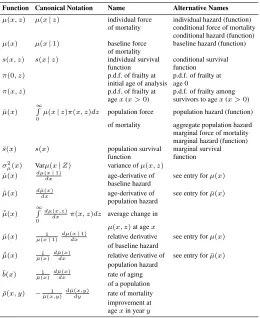
Table A.1: Functions used in the main text (column 1), corresponding standard probability theory notation (column 2), most commonly used name in the main text (column 3), and alternative names (column 4).
Function Canonical Notation Name Alternative Names
µ(x, z) µ(x|z) individual force individual hazard (function) of mortality conditional force of mortality
conditional hazard (function)
µ(x) µ(x|1) baseline force baseline hazard (function) of mortality
s(x, z) s(x|z) individual survival conditional survival function function
π(0, z) p.d.f. of frailty at p.d.f. of frailty at initial age of analysis age 0
π(x, z) p.d.f. of frailty at p.d.f. of frailty among agex(x >0) survivors to agex(x >0)
¯
µ(x)
∞
R
0
µ(x|z)π(x, z)dz population force population hazard (function) of mortality aggregate population hazard marginal force of mortality marginal hazard (function) ¯
s(x) s(x) population survival marginal survival function function
σ2µ(x) Varµ(x|Z) variance ofµ(x, z) ˙
µ(x) dµ(xdx|1) age-derivative of see entry forµ(x) baseline hazard
˙ ¯
µ(x) d¯µ(x)dx age-derivative of see entry forµ¯(x) population hazard
¯˙
µ(x)
∞
R
0 dµ(x,z)
dx π(x, z)dz average change in
µ(x, z)at agex
´
µ(x) 1
µ(x|1) dµ(x|1)
dx relative derivative see entry forµ(x)
of baseline hazard ´
¯
µ(x) 1
¯ µ(x)
d¯µ(x)
dx relative derivative of see entry forµ¯(x)
population hazard ¯
b(x) 1
¯ µ(x)
d¯µ(x)
dx rate of aging
of a population ¯
ρ(x, y) − 1 ¯ µ(x,y)
d¯µ(x,y)
dy rate of mortality