in the population sciences published by the Max Planck Institute for Demographic Research Konrad-Zuse Str. 1, D-18057 Rostock · GERMANY www.demographic-research.org
DEMOGRAPHIC RESEARCH
VOLUME 22, ARTICLE 20, PAGES 579-634
PUBLISHED 13 APRIL 2010
http://www.demographic-research.org/Volumes/Vol22/20/ DOI: 10.4054/DemRes.2010.22.20
Research Article
No consistent effects of prenatal or neonatal
exposure to Spanish flu on late-life mortality
in 24 developed countries
Alan A. Cohen
John Tillinghast
Vladimir Canudas-Romo
© 2010 Alan A. Cohen, John Tillinghast & Vladimir Canudas-Romo.
This open-access work is published under the terms of the Creative Commons Attribution NonCommercial License 2.0 Germany, which permits use, reproduction & distribution in any medium for non-commercial purposes, provided the original author(s) and source are given credit.
1 Introduction 580
2 Methods 582
2.1 Data 582
2.2 Analyses 585
2.2.1 24-country multilevel models 585
2.2.2 Life expectancy 586
2.2.3 France, Italy, and Switzerland: finer-scale cohorts 591
2.2.4 Sensitivity analyses 592
3 Results 593
3.1 Twenty-four-country mortality analysis 593
3.2 Life expectancy 601
3.3 France, Italy, and Switzerland with half-year Lexis pseudo-cohorts 603
4 Discussion 603
4.1 Effects of the flu on late-life mortality 603
4.2 Methodological advances 609
5 Acknowledgments 610
Literature cited 611
Appendix A: Lexis Pseudo-cohort methodology and details 615
Appendix B: A selection of sensitivity analyses 624
No consistent effects of prenatal or neonatal exposure to
Spanish flu on late-life mortality in 24 developed countries
Alan A. Cohen1
John Tillinghast2
Vladimir Canudas-Romo3
Abstract
We test the effects of early life exposure to disease on later health by looking for differences in late-life mortality in cohorts born around the 1918-1919 flu pandemic using data from the Human Mortality Database for 24 countries. After controlling for age, period, and sex effects, residual mortality rates did not differ systematically for flu cohorts relative to surrounding cohorts. We calculate at most a 20-day reduction in life expectancy for flu cohorts; likely values are much smaller. Estimates of influenza incidence during the pandemic suggest that exposure was high enough for this to be a robust negative result.
1 Corresponding author. Current address: Centre de recherche PRIMUS, Universite de Sherbrooke, 3001 12e
Ave Nord, Sherbrooke, QC J1H 1A8, Canada. tel.: (819) 580-2655. fax: (819) 564-5424. E-mail: [email protected].
2 Johns Hopkins University. E-mail: [email protected].
1. Introduction
It has long been hypothesized that events early in life could affect the developmental process and thereby health at later ages. Such effects are well-known in animal models, and have been observed in humans for a number of specific diseases (Barker 1990; Barker 1997; Ozanne 2001). Finch and Crimmins (2004) showed an association between early and late mortality in cohorts from Sweden, and suggest that this could imply an effect on lifespan of high inflammation resulting from infections early in life. However, links between early and late life mortality could also result from famine or other factors not directly related to early inflammation; data on the effects of famine are mixed (Kannisto et al. 1997; Ravelli et al. 1998; Stanner et al. 1997). Generally speaking, disease and malnutrition tend to co-occur, making it hard to tease apart these factors with population data.
One potential way to distinguish effects of disease from malnutrition is to use the Spanish influenza pandemic of 1918-1919. Although following close on the heels of World War I and the potential food shortage accompanying war, the pandemic affected neutral countries as well and did not occur at a time of generalized food shortages more severe than what had occurred in the previous years of the war. Thus, any significant differences in late-life mortality of 1918 and 1919 cohorts relative to surrounding cohorts is likely attributable to the pandemic, especially if such effects can be generalized across countries. Mortality from the pandemic is estimated at 50-100 million worldwide, the largest well-recorded demographic event on record (Johnson and Mueller 2002); while the damage was somewhat less in developed countries, no country was immune and effects were severe even in Denmark, the country with lowest excess mortality (Murray et al. 2006).
life, potentially resulting in high constitutive inflammation levels. There may be other pathways as well by which early exposure to disease could affect late-life mortality.
If early exposure to influenza increases mortality via inflammation pathways, we can make several predictions. To start with, the effect should be strongest in those hit by the flu postnatally, when there is less reliance on the maternal immune system (Holt 1995). In contrast, other pathways should be strongest for prenatal exposure, since disturbance earlier in development is likely to have more severe long-term consequences in most cases. Because the timing of the flu pandemic was precise and roughly synchronized worldwide, with most mortality occurring in fall 1918 followed by a smaller wave in early 1919 (Johnson and Mueller 2002), we should expect 1918 cohort mortality (i.e., mostly those already born before the flu hit) to be higher than 1919 cohort mortality (mostly those still in utero during exposure) if inflammation is the primary pathway of action; conversely, if more general developmental disturbance through under-allocation of maternal resources is the primary pathway, the 1919 cohort should have higher late-life mortality. Also, we would expect a slightly delayed cohort effect in Australia, which managed to delay onset of the flu to early 1919 by a maritime quarantine (Johnson and Mueller 2002).
Potentially confounding these predictions, there are also pathways by which early exposure to disease could actually lower late-life mortality. First, high exposure to disease could cull the weakest infants from a cohort; the survivors should be the most robust individuals and therefore predisposed to live longer. Such selection effects have been documented in wild animals such as Leach’s Storm-Petrel (Oceanodroma leucorhoa) (Mauck et al. 2004). Second, early exposure to disease could actually improve the long-term health of infants. Hunter-gatherers are likely exposed to much higher disease burdens than modern humans and are known to have constitutively high inflammation levels (Gurven et al. 2008). If this is representative of the environment in which our immune systems evolved, it may well be that proper development of the immune system requires exposure to pathogens for some “priming” effect. Along these lines, there are hypotheses that modern epidemics of allergies and asthma result from early under-exposure of the immune system (Folkerts et al. 2000; Holt 1995); it might be reasonable to expect similar such effects in other aspects of the immune system late in life, including auto-immune disease and regulation of inflammation.
economic and health outcomes were poorer for cohorts born in the U.S. during the flu, but mortality has not been examined (Almond 2006; Almond and Mazumder 2005).
Here, we take publicly available data from the online Human Mortality Database to test for differences in late-life mortality between Spanish flu cohorts and surrounding cohorts. We restrict analyses from ages 45 to about 80, depending on country, and to cohorts born between 1911 and 1923. To ensure that all ages tested are included for all cohorts, we limit countries analyzed to those with mortality data dating back to 1956 (= 1911 + 45), a set of 24 countries including most of Europe (but not the Soviet bloc), the U.S., Canada, Australia, Japan, and New Zealand. Details of the data are described in section 2.1. We use residual mortality rates after accounting for age, period, and sex effects; age and period splines are used to account for non-linear trends (see 2.2.1). Life expectancy is also analyzed (see 2.2.2). Finer-scale cohort analyses are performed for France, Italy, and Switzerland (see 2.2.3).
2. Methods
2.1 Data
available countries, 16 had old enough data regardless of first age and cohort used, and two (Slovenia and Taiwan) clearly did not have good coverage at the youngest ages. However, 15 countries had mortality data starting between 1947-1959, which would limit the youngest age and/or earliest cohort used. We ran the analyses with different combinations for all countries and found consistent results; here, we present data using cohorts from 1911 (to include some pre World War I data) starting at age 45. This results in exclusion of Poland and the former Soviet republics; we were not confident in the quality of the Soviet republic data, but there were no clear patterns in these excluded countries that contradict our broader findings. Thus, we used a cohort range of 1911-1923, an age range of 45-~81 (depending on the last year of data available for each country), and a set of 24 countries (Table 1). Roughly 22,000 mortality data points were incorporated into the analyses.
Table 1: Data used for this analysis by country, with World War II mortality estimates
Country Min age Max age Cohort range Earliestperiod
data
WWII mortality (% of 1939 population)a
Australia 45 80 1911-1923 1921 0.57%
Austria 45 81 1911-1923 1947 5.50%
Belgium 45 81 1911-1923 1841 1.02%
Bulgaria 45 81 1911-1923 1947 0.38%
Canada 45 80 1911-1923 1921 0.40%
Czech Republic 45 80 1911-1923 1950 2.25%
Denmark 45 82 1911-1923 1835 0.08%
England and Wales 45 79 1911-1923 1841 0.94%
Finland 45 82 1911-1923 1878 2.62%
France 45 81 1911-1923 1899 1.35%
West Germany 45 80 1911-1923 1956 8.60%
East Germany 45 80 1911-1923 1956 8.60%
Hungary 45 81 1911-1923 1950 6.35%
Italy 45 80 1911-1923 1872 1.02%
Japan 45 82 1911-1923 1947 3.78%
The Netherlands 45 82 1911-1923 1850 3.44%
New Zealand 45 79 1911-1923 1846 0.67%
Norway 45 82 1911-1923 1876 0.32%
Portugal 45 81 1911-1923 1940 0%?b
Slovakia 45 82 1911-1923 1950 2.25%
Spain 45 81 1911-1923 1908 0.02%c
Sweden 45 82 1911-1923 1751 0.03%
Switzerland 45 82 1911-1923 1876 0.00%
USA 45 80 1911-1923 1933 0.32%
aSources: Ellis (1993) and Frumkin (1951) have estimated casualty statistics for many countries and regions. An extensive list can be
found at http://en.wikipedia.org/wiki/World_War_II_casualties.
bCurrently not listed in our sources, but presumably very low, since Portugal was neutral.
2.2 Analyses
2.2.1 24-country multilevel models
Mortality rates (deaths per exposure per year) were log-transformed so that the increase with age was roughly linear. Henceforth we refer to log-mortality rates simply as “mortality rates.” We used regression (general linear models) to calculate residual log-mortality after accounting for age, period, and sex. Year of death (period) was calculated as year of birth plus age at death plus one, which is the average time of death assuming constant fertility rates within each year of birth and constant death rates within each one-year age class. We centered age and period and then calculated polynomial B-spline bases with knots every 10 years (R v. 2.8.1, “splines” package, “bs” function). Weighted least squares Poisson regression models calculated mortality as a function of age splines, period splines, sex, and all two-way interactions among them, and can be represented as:
μ = Σasi + Σysj + sex + Σ(asi×ysj) + Σ(asi×sex) + Σ(ysj×sex) + ε (1)
where μ is log-mortality for a given cohort, age, and sex; asi are centered spline terms
for age at death (summed over all values of i, approximately 5); ysj are centered spline
terms for year of death (summed over all values of j, approximately 6), and ε is the residual mortality. There are thus 53 terms in the full model. We weighted the regression by the number of deaths in each stratum because the expected number of deaths can be shown to be approximately equal to the variance under a Poisson distribution (by the Delta method).
Depending on country, variance explained by this model ranged from 99.51% to 99.95%. Residuals from this model (“residual mortality”) were used in subsequent analyses, and represent mortality after accounting for age, period, and sex effects. The small percentage of variation accounted for by residual mortality is expected given the large changes in mortality with age and period relative to what might be expected from an additional cohort effect. Residual mortality rates were calculated separately for each country using R v. 2.8.1 (R Core Development Team 2007). We checked for patterns of non-randomness in the residuals using mean residuals (across country and sex) plotted against age at death, year of death, and three-dimensional surface plots across Lexis surfaces (Fig. 1).
no need to include terms in the model for country or overall mean. The specified model was:
mr(ijk) = β(k) + ε(ijk) (2) where mr is residual mortality, i is individual mortality data point (for a given age,
cohort, sex, and country), j is country, k is cohort, βs are normally distributed cohort-specific deviations from 0, and ε is a normally distributed error term. Variances of β
and ε were also estimated and assumed to be gamma-distributed. In order to calculate deviations of specific combinations of country and cohort from the overall average, we used a nested cohort-within-country model, similar to equation (2) except with the β2s nested within the β1s:
mr(ijk) = β1(j) + β2(jk) + ε(ijk) (3) Shrunk estimated Bayes values were calculated for each cohort (from equation (1)) and for cohort-country combination (from equation (2)). Multilevel models were fit using Bayesian Gibbs sampling and Markov Chain-Monte Carlo simulations (4000 iterations, first 1000 discarded to allow for convergence) in WinBUGS v. 1.4.3 (Spiegelhalter et al. 2007).
2.2.2 Life expectancy
Figure 1a: Plots of residual log-mortality (after running the age-period-sex model) averaged across country and sex by age
45 50 55 60 65 70 75 80
-0.
005
0.
000
0.
005
Age
M
ean r
es
idual
Figure 1b: Plots of residual log-mortality (after running the age-period-sex model) averaged across country and sex by year
1960 1970 1980 1990 2000
-0
.0
2
-0.
01
0.
00
0
.0
1
0.
02
Year
M
e
an
r
e
si
du
al
Figure 1c: Plots of residual log-mortality (after running the age-period-sex model) averaged across country and sex by age and cohort simultaneously
Age
C oh
ort
M ean
R esid
ual
Figure 1d: Plots of residual log-mortality (after running the age-period-sex model) averaged across country and sex by age and year simultaneously
Year of dea th
A ge M ea n R e sidu
al
2.2.3 France, Italy, and Switzerland: finer-scale cohorts
We took a somewhat different approach to analyzing the finer-scale data from France, Italy, and Switzerland. Because we used Lexis data rather than cohort data, we were able to calculate two mortality rates for each age-cohort-sex-country combination: one for people who died in the earlier possible year, and one for people who died in the later possible year. For example, a woman who was born in 1918 and died at age 60 could have died in 1978 or 1979, depending on when in 1918 she was born and exact age at death. The Lexis data allow us to separate those who died in 1978 from those who died in 1979. The probability of dying in 1978 versus 1979 depends on when in 1918 the woman was born: the closer to the beginning of 1918, the higher the probability she would die in 1978 (given death at age 60). This relationship can be used to calculate distributions of birthdays for those who died in the earlier versus the later possible years. Assuming equal birth rates throughout a year and equal death rates throughout a one-year age class, those dying in the earlier possible year have a mean birthday about May 2, with 75% born in the first half of the year. Those dying in the later possible year have a mean birthday about September 1, with 75% born in the second half. Thus any large differences in mortality rates between half-year cohorts should be apparent (though not precisely estimable) in differences between these “Lexis pseudo-cohorts” – those that died in the earlier versus later possible year, for a given one-year age class and one-year birth cohort. If age is a, and year of birth is c, the two Lexis pseudo-cohorts are thus those who died in year a + c and those who died in year a + c + 1. We will refer to these cohorts as “spring births” and “fall births” respectively, though of course there are individuals in each cohort born at all times of year; the seasons are probabilistic averages. The method is developed at greater length in Appendix A, and details of the above calculations are provided. Related approaches for slightly different contexts have been developed by Bell and Rees (2006).
way through the year. Thus, only 1/24 of their lives are spent exposed to risk in year a + c + 1, and 23/24ths are spent in year a + c. Similarly, for February the proportions are 3/24ths and 21/24ths, etc. The baseline sizes of the spring and fall cohorts can each be calculated as the sum across months of the product of births in that month and the proportion of life lived in year a + c or year a + c + 1, as appropriate for that month and cohort. Full-year exposures can then be allocated to the Lexis pseudo-cohorts not by dividing in half, but by multiplying by the percentage of births that were allocated to each respective Lexis pseudo-cohort. This method does not account for immigration or emigration, and assumes that differences in death rates between the Lexis pseudo-cohorts do not affect cohort sizes; nonetheless, it should yield a reasonable approximation of the exposures for each Lexis pseudo-cohort, allowing calculation of Lexis-cohort-specific death rates (deaths/exposures).
Because the years for which monthly fertility data were available differed between France, Italy, and Switzerland, we ran the countries separately rather than including country as a level in a multilevel model. For each, we generated functions predicting mortality as a function of age and period using splines as outlined above. However, fertility data by month were not sex-specific, so we used total death rates and exposures and do not include a sex term in the model. We then used these functions to generate predicted mortality for each age and year of death; residuals were calculated as the difference between observed and predicted values. We then modeled these residuals as a function of spring versus fall birth (i.e., Lexis pseudo-cohort) and calculated final residual values. Analyses up to this point were conducted in R; we then imported the residuals into WinBUGS, modeling the heterogeneity of residual mortality across cohorts as above but separately for each country (i.e., equation (1) with no β2 terms).
2.2.4 Sensitivity analyses
(equation (3)) and country-within-cohort (equation (4)) models instead of the base model (equation (2)).
mr(ikj) = β1(k) + β2(kj) + ε(ikj) (4) Lastly, we worried that flu cohorts, who would have been young adults during World War II, might have suffered a specific mortality pattern then that could bias our results; for example, if World War II mortality were normally distributed across cohorts with a peak for the 1919 cohort, there could have been culling of the most healthy individuals (i.e., those fit for battle) in a way that would affect our estimates. We addressed this concern by running the multilevel model including only females and by using subsets of countries with low (<0.75%) or very low (<0.1%) mortality during the war (as a percent of 1939 population, Table 1). Again, there were no substantive differences and results are presented in Appendix B.
3. Results
3.1 Twenty-four-country mortality analysis
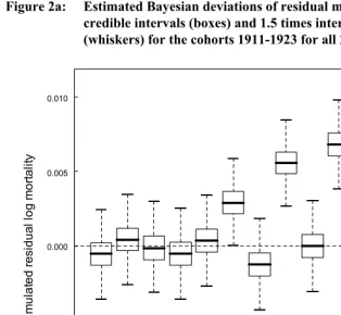
There was little evidence for differences in mortality rates among cohorts (Figure 2a;
β1s from equation (2)), though it is possible that mortality was slightly higher in the 1918 and 1920 cohorts but lower in the 1922 cohort. However, there appears to be substantial heterogeneity across countries within cohorts: out of 312 countries within cohorts, 42 had 95% credible intervals that did not include zero (22 above, 20 below, Figure 3; β2s from equation (3)). False discovery rates are not generally a concern with Bayesian sampling methods.
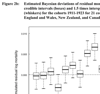
model, both 1918 and 1919 rates are higher than zero and are the two highest observed, but 1922 rates are the farthest from the overall average. Thus, there does appear to be high mortality in the 1918-1919 cohorts (though not outside the range of normal variation), a pattern not seen when all 24 countries are included.
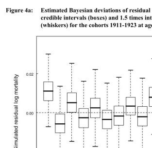
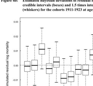
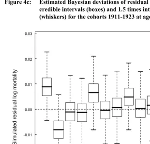
Next, following the suggestion of Bruckner and Catalano (2009) that effects of early disease might be strongest at younger ages, we looked for differences in mean cohort residual mortality for younger age groups, 5-30, 5-45, and 15-45. For the first two analyses, years of available data constrained us to include only 11 countries: Belgium, Denmark, England & Wales, Finland, France, Italy, the Netherlands, Norway, Spain, Sweden, and Switzerland; for the 15-45 analysis we were additionally able to include Australia and Canada. None of the analyses showed appreciable differences in mortality among any of the cohorts 1911-1923 (Figure 4)
Figure 2a: Estimated Bayesian deviations of residual mortality rates with 50% credible intervals (boxes) and 1.5 times interquartile range
(whiskers) for the cohorts 1911-1923 for all 24 countries.
1911 1912 1913 1914 1915 1916 1917 1918 1919 1920 1921 1922 1923 -0.010
-0.005 0.000 0.005 0.010
Cohort
S
im
u
la
te
d r
e
sid
u
al lo
g
m
o
rt
ali
Figure 2b: Estimated Bayesian deviations of residual mortality rates with 50% credible intervals (boxes) and 1.5 times interquartile range
(whiskers) for the cohorts 1911-1923 for 21 countries, excluding England and Wales, New Zealand, and Canada.
1911 1912 1913 1914 1915 1916 1917 1918 1919 1920 1921 1922 1923 -0.010
-0.005 0.000 0.005 0.010
Cohort
S
im
u
lat
e
d r
e
si
d
u
a
l l
o
g m
o
rt
al
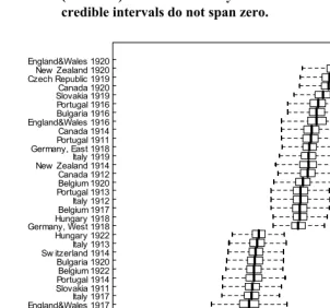
Figure 3: Estimated Bayesian deviations of residual mortality rates with 50% credible intervals (boxes) and 1.5 times interquartile range
(whiskers) for the 42 country-cohort combinations whose 95% credible intervals do not span zero.
England&Wales 1919Canada 1919 New Zealand 1919Portugal 1912 Bulgaria 1915 Czech Republic 1918Norw ay 1917 Slovakia 1922Italy 1922 England&Wales 1917Italy 1917 Slovakia 1911 Portugal 1914Belgium 1922 Bulgaria 1920 Sw itzerland 1914Italy 1913 Hungary 1922 Germany, West 1918Hungary 1918 Belgium 1917Italy 1912 Portugal 1913Belgium 1920 Canada 1912 New Zealand 1914Italy 1919 Germany, East 1918Portugal 1911 Canada 1914 England&Wales 1916Bulgaria 1916 Portugal 1916 Slovakia 1919Canada 1920 Czech Republic 1919New Zealand 1920 England&Wales 1920
-0.10 -0.05 0.00 0.05 0.10
Simulated residual log mortality
Figure 4a: Estimated Bayesian deviations of residual mortality rates with 50% credible intervals (boxes) and 1.5 times interquartile range
(whiskers) for the cohorts 1911-1923 at ages 5-30.
1911 1912 1913 1914 1915 1916 1917 1918 1919 1920 1921 1922 1923 -0.02
0.00 0.02
S
im
u
lat
ed
r
es
idual
log
m
or
tal
ity
Figure 4b: Estimated Bayesian deviations of residual mortality rates with 50% credible intervals (boxes) and 1.5 times interquartile range
(whiskers) for the cohorts 1911-1923 at ages 5-45.
1911 1912 1913 1914 1915 1916 1917 1918 1919 1920 1921 1922 1923 -0.03
-0.02 -0.01 0.00 0.01 0.02 0.03
S
im
u
la
ted r
e
si
dual
log m
o
rt
al
ity
Figure 4c: Estimated Bayesian deviations of residual mortality rates with 50% credible intervals (boxes) and 1.5 times interquartile range
(whiskers) for the cohorts 1911-1923 at ages 15-45.
1911 1912 1913 1914 1915 1916 1917 1918 1919 1920 1921 1922 1923 -0.02
-0.01 0.00 0.01 0.02 0.03
S
im
u
la
ted r
e
si
dual
log m
o
rt
al
ity
3.2 Life expectancy
Life expectancy analyses confirmed the results of the mortality analysis (Figure 5). There were marginal negative effects of being born in 1918 or 1919, particularly when England and Wales, New Zealand, and Canada were excluded from the analyses (Figure 5b). However, there were positive effects on life expectancy of similar magnitude in 1914 and 1922. Males and females showed similar patterns across years (Pearson’s r=0.83), though patterns in females seemed stronger. The largest effect
Figure 5a: Mean residual life expectancy for ages 45-79 by cohort and sex, averaged across countries for all 24 countries.
observed was for females born in 1919 excluding the three Commonwealth countries, about 19 days less life expectancy. If we extrapolate that roughly half of babies born in 1919 were in utero for substantial periods when the pandemic was raging, that roughly one-third of these were actually exposed to the flu, and that all of the 1919 effect is attributable to the pandemic, we can calculate that life expectancy is lowered 114 days by exposure to the flu in utero. However, this is a maximum estimate: it is not clear that the low life expectancy of the 1919 cohort is any different than might be expected based on random yearly variation (as opposed to the flu) nor that we should exclude the Commonwealth countries, and even if the effect is real the estimate for males is only about half as large.
Figure 5b: Mean residual life expectancy for ages 45-79 by cohort and sex, averaged across countries for 21 countries excluding England and Wales, New Zealand, and Canada
3.3 France, Italy, and Switzerland with half-year Lexis pseudo-cohorts
Using the Lexis pseudo-cohorts described above and the appropriate adjustments for fertility throughout birth year, we were able to test for differences in mortality across half-year cohorts, potentially detecting effects of the influenza pandemic on late-life mortality that are not apparent at a one-year time scale. As in the above analysis, some cohorts in some countries had mortality that differed significantly from the overall average for that country (Figure 6). Across the three countries, there is no consistent trend for high or low mortality in the three cohorts of primary interest (second half of 1918, both halves of 1919). In France (Figure 6a) all three cohorts have 95% credible intervals spanning zero, and in Italy (Figure 6b) the first half of 1919 appears to have low mortality but is well within the range of variation seen across other cohorts. In Switzerland (Figure 6c), the second half of 1918 and first half of 1919 have high mortality and the second half of 1919 has low mortality, with the latter two cohorts having the largest mean differences from the overall average of any cohorts in any of the three countries. However, the magnitude of the deviance is similar for both, and we cannot exclude the possibility that the apparent effect is due to some estimation problem of the proper cohort sizes for that year. A similar issue could account for the symmetrically high and low mortality rates of the two 1921 cohorts in Italy.
4. Discussion
4.1 Effects of the flu on late-life mortality
Figure 6a: Estimated Bayesian deviations of residual mortality rates with 50% credible intervals (boxes) and 1.5 times interquartile range
(whiskers) for France 1914-1919.
1914 a 1914 b 1915 a 1915 b 1916 a 1916 b 1917 a 1917 b 1918 a 1918 b 1919 a 1919 b -0.10 -0.05 0.00 0.05 0.10
France: Residual mortality ranges of cohorts
Figure 6b: Estimated Bayesian deviations of residual mortality rates with 50% credible intervals (boxes) and 1.5 times interquartile range
(whiskers) for Italy 1911-1923.
19 11 a 19 11 b 19 12 a 19 12 b 19 13 a 19 13 b 19 14 a 19 14 b 19 15 a 19 15 b 19 16 a 19 16 b 19 17 a 19 17 b 19 18 a 19 18 b 19 19 a 19 19 b 19 20 a 19 20 b 19 21 a 19 21 b 19 22 a 19 22 b 19 23 a 19 23 b -0.10 -0.05 0.00 0.05 0.10
Italy: Residual mortality ranges of cohorts
Figure 6c: Estimated Bayesian deviations of residual mortality rates with 50% credible intervals (boxes) and 1.5 times interquartile range
(whiskers) for Switzerland 1910-1923.
19 10 a 19 10 b 19 11 a 19 11 b 19 12 a 19 12 b 19 13 a 19 13 b 19 14 a 19 14 b 19 15 a 19 15 b 19 16 a 19 16 b 19 17 a 19 17 b 19 18 a 19 18 b 19 19 a 19 19 b 19 20 a 19 20 b 19 21 a 19 21 b 19 22 a 19 22 b 19 23 a 19 23 b -0.10 -0.05 0.00 0.05 0.10
Switzerland: Residual mortality ranges of cohorts
There was potential evidence of an effect of the pandemic on late-life mortality when we excluded three Commonwealth countries with apparently spurious data – England and Wales, New Zealand, and Canada – from the analysis. (More detail on why we distrust the data from these countries is available in Appendix C.) The trend was still not significant at α=0.05 and the effect was small (less than 20 days lost life expectancy for females born in 1919), but we cannot exclude the possibility of a weak effect. There was also high mortality in Switzerland for those born in the second half of 1918 and first half of 1919, but low mortality for those born in the second half of 1919. This would be consistent with negative effects on the long-term health of neonates but a selection effect on those early in utero during the pandemic. However, the symmetry of the 1919 effects suggests they could also be attributable to the same error in estimating the relative sizes of those cohorts that we believe biased the estimates in the three Commonwealth countries. Similar effects were not apparent in France or Italy, so it would be premature to draw any strong conclusions from the Swiss data. Moreover, the Swiss data do not confirm the Commonwealth-excluded analysis because the effects for the two halves of 1919 cancel each other out: none of the three countries we examined with Lexis pseudo-cohorts bolsters the case for a weak overall 1919 effect.
Our results stand in contrast to several studies showing long-term effects of the flu. Azambuja (2004) and Mamelund (2003) showed potential negative health consequences for those who were adults or young adults when the pandemic hit. However, the lack of clear age specificity of such proposed effects makes it hard to fully distinguish period and cohort effects, and the trends must remain suggestive rather than conclusive of the flu as a causal mechanism. Mazumder et al. (2009), showed apparent effects of the pandemic on cardiovascular disease and adult height for those born around that time, particularly in early 1919. In a careful analysis incorporating both quarter of birth and state, Almond (2006) showed consistently poorer outcomes for the flu cohorts in the 1960, 1970, and 1980 U.S. censuses on economic measures including educational attainment, annual income, neighbors’ income, and disability status. A similar analysis of health outcomes such as self-reported health, history of stroke or diabetes, and functional impairment also found some worse outcomes for flu cohorts, but in many cases the effects were not consistent among flu cohorts born in different quarters, even for relatively similar measures such as Trouble Lifting or Trouble Walking At All (Almond and Mazumder 2005). Because worse economic and health outcomes should lead to higher mortality, it is somewhat surprising that we did not detect such effects in mortality.
There are several potential explanations for the discrepancy between our results and these other studies. First, many of the economic outcomes could be determined by factors earlier in life: educational attainment, for example, is almost certainly not caused by health later in life, since nearly all individuals in these cohorts would have reached their maximum level of education by their mid-twenties. While it is conceivable that early health status could affect both educational attainment and late-life health, there is not a requisite causal link. Second, if the causal pathway is Poor Early Health → Low Educational Attainment → Low Economic Status → Poor Health
→ High Mortality, or something similar, we should expect the effects to be diluted with each successive causal link (arrow), with the link to mortality being hardest to detect. Third, mortality is a composite of many processes, and it is quite possible that countervailing effects might average themselves out here (e.g., lower cancer rates but higher heart disease) in ways that are not predicted by the economic measures. Fourth, it is possible there was a real effect in the U.S. but no effect in all the countries aggregated together. In the U.S. mortality was significantly higher in the 1918 cohort (t=6.67, p<0.0001) and lower in the 1919 cohort (t=-3.65, p=0.0005) compared to all other cohorts. There was no net effect pooling the two cohorts (t=1.08, p=0.28), but the 1918 effect was larger, potentially indicating a pattern in the U.S. that we missed by using one-year cohorts.
Switzerland, many of the cohorts had mortality significantly above or below average. Forty-two of 312 country-cohort combinations also had mortality above or below the overall average. There was also significant heterogeneity in mortality across cohorts in our base model (Fig. 1). Lastly, the strong correlation between cohort-specific male and female life expectancy suggests real trends rather than random deviations. It is possible that the cohort effects are an artifact of imperfect control for age and period, but given that we detect them in multiple analyses and that our age-period-sex model explained more than 99% of the variation, we view this as unlikely. Real cohort effects are not likely attributable to events later in life, since there are few events that would discretely affect one age-class but not another adjacent to it. The events that do have such discrete effects are almost always legal in nature and thus not generalizable across countries. The cohort effects we detect are thus likely attributable to environmental factors very early in life. It is paradoxical that we detected no specific effect of the flu, one of the most salient early-life environmental factors on record, but detected more general evidence for such effects operating at a very fine scale. It is not clear what sorts of variation are causing these cohort effects.
4.2 Methodological advances
mortality as an outcome variable in regression models means that any characteristic which varies across cohorts can be tested or controlled for its effects on cohort mortality.
Some properties of the model require further exploration. In particular, we tested the residuals of the spline model for autocorrelation with respect to age and period. There was a significant period autocorrelation at lag 1, probably indicating that there is continuity in patterns over time. There were also significant age autocorrelations at lags of three, four, seven, and nine. We believe these arise through effects of the spline models, and that, rather than creating statistical problems, correcting for them with a generalized least squares model could actually bias our results by skewing the way the splines operate. However, confirming this will require validation studies beyond the scope of this study.
Finally, we believe that the Lexis pseudo-cohort approach we developed here may be useful in other situations for distinguishing finer-scale cohorts than are initially apparent in the data. For example, several studies have shown that fall babies have higher life expectancy than spring babies (the “Doblhammer effect,” Doblhammer 2004; Doblhammer and Vaupel 2001), but because linked birth and date-of-death data are hard to acquire, the effect has only been shown in several countries. A Lexis pseudo-cohort approach should be able to substantially increase the number of countries and time periods for which inferences can be made, allowing analysis of historical trends in the strength and distribution of this effect. We are currently pursuing these analyses.
5. Acknowledgments
Literature cited
Almond, D. (2006). Is the 1918 influenza pandemic over? Long-term effects of in utero influenza exposure in the post-1940 U.S. population. Journal of Political Economy 114(4): 672-712. doi:10.1086/507154.
Almond, D. and Mazumder, B. (2005). The 1918 influenza pandemic and subsequent health outcomes: An analysis of SIPP data. American Economics Review 95(2): 258-262. doi:10.1257/000282805774669943.
Azambuja, M.I.R. (2004). Spanish flu and early 20th-century expansion of a coronary heart disease-prone subpopulation. Texas Heart Institute Journal 31: 14-21. Barker, D.J.P. (1990). The fetal and infant origins of adult disease. British Medical
Journal 301: 1111. doi:10.1136/bmj.301.6761.1111.
Barker, D.J.P. (1997). The fetal origins of coronary artery disease. European Heart Journal 18: 883-884.
Bell, M. and Rees, P. (2006). Comparing migration in Britain and Australia: harmonisation through use of age – time plans. Environment and Planning A 38(5): 959–988. doi:10.1068/a35245.
Bruckner, T.A., and Catalano, R.A. (2009). Infant mortality and diminished entelechy in three European countries. Social Science and Medicine 68(9): 1617-1624.
doi:10.1016/j.socscimed.2009.02.011.
Calot, G. (1998). Two centuries of Swiss demographic history. Neuchâtel and Paris: Swiss Federal Statistical Office and Observatoire démographique européen. Caselli, G. and Capocaccia, R. (1989). Age, period, cohort and early mortality: An
analysis of adult mortality in Italy. Population Studies 43(1): 133-153.
doi:10.1080/0032472031000143886.
Crimmins, E.M. and Finch, C.E. (2006). Infection, inflammation, height, and longevity. Proceedings of the National Academy of Sciences (USA) 103(2): 498-503.
doi:10.1073/pnas.0501470103.
Crosby, A.W. (1990). America’s forgotten pandemic: the influenza of 1918. New York: Cambridge University Press.
Doblhammer, G. and Vaupel, J.W. (2001). Lifespan depends on month of birth. Proceedings of the National Academy of Sciences (USA) 98(5): 2934-2939.
doi:10.1073/pnas.041431898.
Ellis, J. (1993). World War II - A statistical survey. New York: Facts on File.
Finch, C.E. and Crimmins, E.M. (2004). Inflammatory Exposure and Historical Changes in Human Life-Spans. Science 305(5691): 1736-1739.
doi:10.1126/science.1092556.
Folkerts, G., Walzl, G., and Openshaw, P.J.M. (2000). Do common childhood infections ‘teach’ the immune system not to be allergic? Immunology Today 21(3): 118-120. doi:10.1016/S0167-5699(00)01582-6.
Frumkin, G. (1951). Population Changes in Europe Since 1939. London: Allen & Unwin.
Gurven, M., Kaplan, H., Winking, J., Finch, C.E., and Crimmins, E.M. (2008). Aging and Inflammation in Two Epidemiological Worlds. The Journals of Gerontology Series A 63(2): 196-199.
Holt, P.G. (1995). Postnatal maturation of immune competence during infancy and childhood. Pediatric Allergy and Immunology 6(2): 59-70.
doi:10.1111/j.1399-3038.1995.tb00261.x.
Horiuchi, S. (1983). The long-term impact of war on mortality: old-age mortality of the First World War survivors in the Federal Republic of Germany. Population Bulletin of the United Nations 15: 80-92.
Huber, M. (1931). La Population de la France Pendant la Guerre. New Haven, CT: Yale University Press.
Human Mortality Database (HMD). University of California, Berkeley (USA), and Max Planck Institute for Demographic Research (Germany).
Johnson, N.P.A.S. and Mueller, J. (2002). Updating the accounts: global mortality of the 1918–1920 “Spanish” influenza pandemic. Bulletin of Historical Medicine 76(1): 105–115. doi:10.1353/bhm.2002.0022.
Mamelund, S.-E. (2003). Effects of the Spanish influenza pandemic of 1918-19 on later life mortality of Norwegian cohorts born about 1900. Oslo: Department of Economics, University of Oslo.
Mamelund, S.-E. (2004). Can the Spanish influenza pandemic of 1918 explain the baby boom of 1920 in neutral Norway? Population 59(2): 229-260.
doi:10.2307/3654904.
Mauck, R.A., Huntington, C.E., and Grubb, T.C. (2004). Age-specific reproductive success: evidence for the selection hypothesis. Evolution 58(4): 880-885.
Mazumder, B., Almond, D., Park, K., Crimmins, E.M., and Finch, C.E. (2010). Lingering prenatal effects of the 1918 influenza pandemic on cardiovascular disease. Journal of Developmental Origins of Health and Disease 1(01): 26-34.
doi:10.1017/S2040174409990031.
Mortara, G. (1925). La Salute Pubblica in Italia Durante e Dopo la Guerra. New Haven, CT: Yale University Press.
Murray, C.J.L., Lopez, A.D., Chin, B., Feehan, D., and Hill, K.H. (2006). Estimation of potential global pandemic influenza mortality on the basis of vital registry data from the 1918–20 pandemic: a quantitative analysis. Lancet 368(9554): 2211-2218. doi:10.1016/S0140-6736(06)69895-4.
Myrskylä, M. (2008) The effects of shocks in early life mortality on later life expectancy and mortality compression: A cohort analysis. Demographic Research 22(12): 289-320. doi:10.4054/DemRes.2010.22.12.
Noymer, A. and Garenne, M. (2000). The 1918 influenza epidemic's effects on sex differentials in mortality in the United States. Population and Develiopment Review 26(3): 565-581. doi:10.1111/j.1728-4457.2000.00565.x.
Ozanne, S.E. (2001). Diabetes in Old Male Offspring of Rat Dams Fed a Reduced Protein Diet. International Journal of Experimental Diabetes Research 2(2): 139-143. doi:10.1155/EDR.2001.139.
R Core Development Team (2007). A Language and Environment for Statistical Computing, version 2.8.1.R Foundation for Statistical Computing, Vienna, Austria.
Spiegelhalter, D., Thomas, A., Best, N., and Lunn, D. (2007). WinBUGS, version 1.4.3. http://www.mrc-bsu.cam.ac.uk/bugs.
Stanner, S.A., Bulmer,K., Andrès, C., Lantseva, O.E., Borodina, V., Poteen, V.V., and Yudkin, J.S. (1997). Does malnutrition in utero determine diabetes and coronary heart disease in adulthood? Results from the Leningrad siege study, a cross sectional study. British Medical Journal 315: 1342–1348.
Stearns, S.C. (1989). The evolutionary significance of phenotypic plasticity: phenotypic sources of variation among organisms can be described by developmental switches and reaction norms. BioScience 39(7): 436-445. doi:10.2307/1311135. Yang, Y. (2006). Bayesian Inference for Hierarchical Age-Period-Cohort Models of
Repeated Cross-Section Survey Data. Sociological Methodology 36(1): 39-74.
Appendix A:
Lexis Pseudo-cohort methodology and details
Traditional demographic analyses often rely on making a clear choice between using period and cohort analyses. If we have data on death year and age at death, we have period data; if we have data on birth year and age we have cohort data (Figure A1). The difference arises because a person born in year c (say, 1918) who dies at age a (say, 60) could die in either year a+c or a+c+1 (1978 or 1979), depending on when the birthday fell in the birth year and how close the person made it to age a+1. For example, someone dying at age 60.95 is still recorded as dying at age 60, but probably died in 1979. When we wish to assess the effect of being born in a given year, we use cohort data; when we wish to assess the effect of events during a year on deaths across age-classes, we use period data.
Figure A1: Lexis diagram of what is known with cohort and age at death (“Cohort data” from the Human Mortality Database).
1920 1919 60
61
A ge
The problem that can arise here is one of scale of the divisions among cohorts, periods, or age classes. We might wish to detect a pattern with a clear threshold point that may be partway through a year, or with cyclical effects operating more rapidly than can be detected by dividing the data up by year. So we’d like half-year cohorts (Figure A2). If we have only period and cohort data by year, there is generally no way to get information on a finer scale. However, sometimes we have Lexis data available, in which case both birth year and death year are present. This provides some additional information that we should be able to utilize for detection of finer scale patterns (Figure A3); the topic of this appendix is how to maximize the information we can gain by utilizing Lexis data.
Figure A2: A Lexis diagram of what we’d like to know: half-year cohorts, with those born in the first half of 1918 in blue and those born in the second half in red.
61
Age
1918 60
Birth year 1919 1920
Figure A3: Lexis diagram of what is known with cohort, year of death, and age at death (“Lexis data” from the Human Mortality Database). Blue shows those born in 1918, dying in 1978, at age 60. Red shows those born in 1918, dying in 1979, at age 60.
Birth
At first glance, it is not immediately apparent how we can get more information. For example, our 1918-born 60-year-old can now be definitively assigned to, say, 1979 as a death year, but we cannot say with certainty when in 1918 she was born or when in 1979 she died. She could have been born early in 1918 (if she died even earlier in 1979) or have died late in 1979 (if she was born even later in 1918). So, unlike our source data, we cannot use absolute knowledge of birth or death at finer scale than a year; at best, we can get probabilistic information.
However, the probabilistic information should be relatively accurate, especially if we make two assumptions: (1) that there are roughly equal numbers of births on each day of a year, and (2) that specific mortality rates are constant throughout an age-class (e.g., chance of dying at 60.00 is the same as at 60.99). Of course, neither assumption is strictly true, but they are both approximately true, and as we will see their violation should not undermine the validity of our analysis under most circumstances. The first assumption allows us to simplify the calculation of the probability of having been born in the earlier or later possible half-year cohort, given age at death and year of death – if numbers of births vary by season, so will the probability of having been born in a given season. The second assumption also helps simplify calculation. If death rates vary within age classes (presumably increasing with age), an individual dying in year a
year
1918 1919 1920
60 61
Age
+ c + 1 will be more likely to have been born in the second half of year c than otherwise expected because being born in the first half would imply having survived a greater fraction of year a than being born in the second, and the chance of this goes down if mortality rates increase with age within a.
The basic insight that allows us to get probabilistic information is that a person born on Jan. 1 of a year is much more likely to die in the first than the second possible death year. If our example subject were born Jan. 1, 1918 the only way she could die in 1979 at age 60 would be to die on Jan. 1 earlier in the day than the time she was born – highly unlikely relative to the probability of dying sometime in 1978. Given that we only know her age at death to the year, we can calculate this probability. If we know that she was born on Jan. 1, 1918 at 11:59 pm and died at age 60, there is a 1/365 chance that she died in 1979 and a 364/365 chance that she died in 1978 (again, assuming constant death rates from age 60.00 to age 60.99). If she were born on Jan. 2 at 11:59 pm, these probabilities would shift to 2/365 and 363/365 respectively, and so on. The probabilities always sum to 1, of course, and they are linear probability density functions of birth date within a year,
PDF = 1-x/365 (1)
PDF = x/365 (2)
Figure A4: Probability of different Julian birthdays (i.e., days in the year numbered 1-365) for those dying in the earlier or later possible year for a given age and cohort.
0 0.1 0.2 0.3 0.4 0.5 0.6 0.7 0.8 0.9 1
0 100 200 300
Julian birthday
P
rob
a
bilit
y
Died in second year Died in first year
All we know from our Lexis data is that someone died in the earlier or later of the two possible years. However, even with just this knowledge, we can establish the probability distributions of date of birth for these two groups as the lines in Figure A4. As can be seen, these distributions overlap but are markedly different. The mean date of birth for those who died in the first year is approximately May 2 (1/3 of the way through the year) and for those who died in the second year is approximately Sept. 1 (2/3 of the way through the year). The expected birthday (in Julian days) can be calculated like the expected value for any random variable,
E(x) = ∫x*f(x)dx (3)
We thus can effectively create two probabilistic pseudo-cohorts with known mean birthdays, what we call “Lexis pseudo-cohorts.” For our purposes, we define Lexis pseudo-cohorts as Lexis triangles (and the data pertaining thereto) when they are used to make probabilistic inferences about the half-scale cohorts with which they overlap 75%. If we conduct analyses on these Lexis pseudo-cohorts, we can now see patterns that emerge at finer scales than one year (Figure A5). Our precision will of course not be as good as if we had two distinct cohorts born with certainty in the first and second half of the year (the precision is 75%, to be precise, Figure A5), but if the effects we are looking for are strong enough we should still be able to detect them.
Figure A5: A Lexis diagram of the 75% overlap between the “Lexis pseudo-cohorts” and true half-year cohorts
61
Age
1918 60
Birth year 1919 1920
1978 Death year 1979 1980
.
Relaxing the assumptions
One assumption of the probability distributions for our two cohorts is that there is no seasonality to birth rates. However, seasonality of births will not affect the probability of each year of death for a given birthday; it affects only the distribution of the birthdays within a year. This is easily incorporated into a model. Figure A6 uses a cosine function to illustrate the sort of effect seasonality could have on our probability distributions. A less symmetric seasonality could bias the original estimates somewhat (Figure A7). In all cases, seasonality could affect estimates of mean birthday for the two cohorts, but should not be strong enough to change the fundamental difference between an earlier and a later cohort that are approximately 50% distinct.
Figure A6: Probability of different Julian birthdays (i.e., days in the year numbered 1-365) for those dying in the earlier or later possible year for a given age and cohort assuming seasonality of birth following a cosine function symmetrical around mid-year (dark blue). The pink and yellow lines are the cosine function multiplied by the linear probability density functions depicted in Figure A4.
0 0.2 0.4 0.6 0.8 1 1.2
0 100 200 300
Julian Birthday
P
roba
bilit
y
Figure A7: Probability of different Julian birthdays (i.e., days in the year numbered 1-365) for those dying in the earlier or later possible year for a given age and cohort assuming seasonality of birth following a sine function that is not symmetrical around mid-year (dark blue). The pink and yellow lines are the sine function multiplied by the linear probability density functions depicted in Figure A4.
0 0.2 0.4 0.6 0.8 1 1.2
0 100 200 300
Julian birthday
P
roba
bi
lit
y
Seasonality of birth Died in second year Died in first year
Figure A8: Probability of different Julian birthdays (i.e., days in the year numbered 1-365) for those dying in the earlier or later possible year for a given age and cohort assuming a 5% difference in allocation of births between the beginning and end of the year, based on the slightly higher probability of death at older ages (dark blue). The pink and yellow lines are the linear decline in birth probability (equivalent to a linear decline in mortality by age within an age class, dark blue) multiplied by the linear probability density functions depicted in Figure A4.
0 0.2 0.4 0.6 0.8 1 1.2
0 100 200 300
Julian birthday
P
rob
a
b
ilit
y Seasonality of birth
Appendix B:
A selection of sensitivity analyses
Figure B1a: Estimated Bayesian deviations of residual mortality rates with 50% credible intervals (boxes) and 1.5 times interquartile range
(whiskers) for the cohorts 1911-1923 for ages 45-70 for all 24 countries.
1911 1912 1913 1914 1915 1916 1917 1918 1919 1920 1921 1922 1923 -0.010
-0.005 0.000 0.005 0.010
S
im
u
la
ted r
e
si
dua
l l
og m
o
rt
al
Figure B1b: Estimated Bayesian deviations of residual mortality rates with 50% credible intervals (boxes) and 1.5 times interquartile range
(whiskers) for the cohorts 1911-1923 for ages 45-70 for 21 countries, excluding England and Wales, New Zealand, and Canada.
1911 1912 1913 1914 1915 1916 1917 1918 1919 1920 1921 1922 1923 -0.010
-0.005 0.000 0.005 0.010 0.015
Cohort
S
im
u
la
te
d
r
e
si
du
al
lo
g m
o
rt
al
Figure B1c: Estimated Bayesian deviations of residual mortality rates with 50% credible intervals (boxes) and 1.5 times interquartile range
(whiskers) for the cohorts 1911-1923 for ages 60-80 for all 24 countries.
1911 1912 1913 1914 1915 1916 1917 1918 1919 1920 1921 1922 1923 -0.010
-0.005 0.000 0.005 0.010
S
im
u
la
te
d
r
e
si
du
al
lo
g m
o
rt
al
Figure B1d: Estimated Bayesian deviations of residual mortality rates with 50% credible intervals (boxes) and 1.5 times interquartile range
(whiskers) for the cohorts 1911-1923 for ages 60-80 for 21 countries, excluding England and Wales, New Zealand, and Canada.
1911 1912 1913 1914 1915 1916 1917 1918 1919 1920 1921 1922 1923 -0.005
0.000 0.005 0.010
Cohort
S
im
u
la
te
d r
e
si
du
al
lo
g
m
o
rt
al
Figure B2a: Estimated Bayesian deviations of residual mortality rates with 50% credible intervals (boxes) and 1.5 times interquartile range
(whiskers) for females only in the cohorts 1911-1923 for all 24 countries.
1911 1912 1913 1914 1915 1916 1917 1918 1919 1920 1921 1922 1923 -0.010
-0.005 0.000 0.005 0.010
S
im
u
la
te
d r
e
si
du
al
lo
g
m
o
rt
al
Figure B2b: Estimated Bayesian deviations of residual mortality rates with 50% credible intervals (boxes) and 1.5 times interquartile range
(whiskers) for females only in the cohorts 1911-1923) for 21
countries, excluding England and Wales, New Zealand, and Canada.
1911 1912 1913 1914 1915 1916 1917 1918 1919 1920 1921 1922 1923 -0.010
-0.005 0.000 0.005 0.010
Cohort
S
im
u
la
te
d
r
e
si
du
al
lo
g m
o
rt
al
Figure B3: Estimated Bayesian deviations of residual mortality rates with 50% credible intervals (boxes) and 1.5 times interquartile range
(whiskers) for the cohorts 1911-1923 in the ten countries in our sample with low (<0.5%) mortality during World War II: Australia, Bulgaria, Canada, Denmark, New Zealand, Norway, Portugal, Sweden, Switzerland, and USA
1911 1912 1913 1914 1915 1916 1917 1918 1919 1920 1921 1922 1923 -0.010
-0.005 0.000 0.005 0.010 0.015
S
im
u
la
te
d r
e
si
du
al
lo
g
m
o
rt
al
Figure B4: Estimated Bayesian deviations of residual mortality rates with 50% credible intervals (boxes) and 1.5 times interquartile range (whiskers) for the cohorts 1911-1923 in the four countries in our sample with very low (<0.1%) mortality during World War II: Denmark, Portugal, Sweden, and Switzerland.
1911 1912 1913 1914 1915 1916 1917 1918 1919 1920 1921 1922 1923 -0.020
-0.015 -0.010 -0.005 0.000 0.005 0.010 0.015
S
im
u
la
te
d
r
e
si
d
ual
log m
o
rt
a
lit
Appendix C:
Adjacent-bias artifacts
When we first started this project, we ran a series of preliminary analyses. One such analysis was to create pseudo-cohorts from period data in the Human Mortality Database (HMD) by subtracting age-at-death from year-of-death. While this is not a method we would seek to defend, it produced a striking result: in almost every country, mortality at older ages for the 1919 cohort was far lower than for any other cohort, and mortality for the 1920 cohort was far higher. Our pseudo-cohorts differed from actual cohorts in that they (a) had a mean birthday at Jan. 1, not halfway through the year, (b) had a range of birthdays that spans two years, not one, and (c) had a higher concentration of birthdays close to the center of the range rather than a uniform distribution. Based on this, we suspected that there was some protective effect of the flu on the very young in most cases (those born in the 1919 pseudo-cohort), but that those exposed very early in pregnancy (i.e., born in the second half of 1919 and thus likely in the 1920 pseudo-cohort) might have suffered severely. We then discovered that this is a known artifact in the HMD (John R. Wilmoth, personal communication).
It is easy for such an artifact to arise when there is some confusion as to the allocation of either deaths or exposures between adjacent cohorts. For example, if a portion of the 1920 population is mistakenly allocated to 1919 but the death counts remain the same, the 1919 cohort mortality rates will appear low while the 1920 rates appear high. The biases should be of similar magnitude but in opposite directions. While such patterns can also be due to real phenomena – for example, periods of low birth rates are often followed by a baby boom – in most cases it is unusual to have symmetrically opposed effects in adjacent cohorts. This can thus serve as a check on data quality and the accuracy of the analysis: symmetrically opposed effects in adjacent cohorts should be treated with suspicion. In the data presented here, we notice such effects in several cases. In the three Commonwealth countries England and Wales, New Zealand, and Canada, we see low mortality in the 1919 cohorts and high mortality in the 1920 cohort. In Switzerland, we see high mortality for the spring 1919 cohort and low mortality for the fall 1919 cohort. In Italy, we see high mortality in the spring 1921 cohort and low mortality in the fall 1921 cohort. In the case of Italy, there is good reason to suspect just such an allocation: the birth-rate calibration we used was with birth rates averaged across the years 1921-23, and a deviation from the average in 1921 would produce just this effect.