Stability and numerical approximation for a spacial class of semilinear parabolic equations on the Lipschitz bounded regions: Sivashinsky equation

Stability and numerical approximation for a spacial class of

semilin-ear parabolic equations on the Lipschitz bounded regions:

Sivashin-sky equation

Mehdi Mesrizedeh Department of mathematics,

Imam Khomeini International University, Qazvin, Iran.

E-mail: [email protected]

Kamal Shanazari∗ Department of mathematics,

University of Kurdistan, Sanandaj, Iran.

E-mail: [email protected]

Abstract This paper aims to investigate the stability and numerical approximation of the Sivashinsky equations. We apply the Galerkin meshfree method based on the radial basis functions (RBFs) to discretize the spatial variables and use a group presenting scheme for the time discretization. Because the RBFs do not generally vanish on the boundary, they can not directly approximate a Dirichlet boundary problem by Galerkin method. To avoid this difficulty, an auxiliary parametrized technique is used to convert a Dirichlet boundary condition to a Robin one. In addition, we extend a stability theorem on the higher order elliptic equations such as the bihar-monic equation by the eigenfunction expansion. Some experimental results will be presented to show the performance of the proposed method.

Keywords. Eigenvalue, Eigenfunction, Galerkin meshless method, Sivashinsky equation, Stability.

2010 Mathematics Subject Classification. 13D45, 39B42.

1. _Introduction

The approximate solution of the Galerkin method is to determine the solution of a system of equations obtained by the variational formulation of the main problem. Also the key property of the Galerkin approach is that the error is orthogonal to the chosen subspaces. In the variational formulation, it is almost always necessary to estimate some integrals. This method has also more computational cost than the collocation method, but it is a stable algorithm and well computes the approximate solution of the well-posed problems. Although it has suffered from deficiencies, special techniques can be used to alleviate the defects in the applications.

Investigated by authors of [6], a set of background cells were required to evaluate the integrals resulted from the use of the Galerkin weak-form. Global numerical integrations were needed to obtain the coefficient matrix of the equation system. Hence, a global background cell structure had to be used for these integrations, so

∗Corresponding author.

that the method was not truly meshless. Also, emphasis was placed on the relationship between the supports of the shape functions and the sub-domains used to integrate the discrete equations. It was shown that constructing the quadrature cells with no attention to the local supports of the shape functions may result in the considerable integration error. They employed the conventional Gauss quadrature rules in the cells for which the high order quadrature rule was needed for sufficient accuracy in the Galerkin meshfree method. Nodal integration, on the other hand, led to rank instability and significant loss of accuracy in the numerical solution. In contrast with using background meshes for integration, discussed above, a truly meshfree Galerkin computational method rely chiefly on the nodal integration maintaining the meshfree characteristics of the weak forms.

The Sivashinsky differential equation, which models a planar solid-liquid interface for a binary alloy fora= 0, is considered as the following nonlinear biharmonic equation [6,4,12]

ut+ ∆2u−a∆u+b u=−∆f(u), in Ω,

u= 0, ∆u= 0, on ∂Ω,

u(0) =u◦, on Ω¯.

(1.1)

where a, b are two positive real numbers, Ω is a bonded Lipschitz region with its boundary∂Ω, andu◦,andf satisfy suitable conditions. This problem was surveyed

and solved by the numerical method given in [9,10]. Dehghan [6] applied the meshless weak form techniques based on the radial point interpolation method for solving this equation and derived an error estimation of its global weak form.

In this work, we apply the Galerkin meshfree method based on the RBFs to the Sivashinsky equation and consider the stability of this equation by the eigenfunction expansion. This paper is organized as follows. In section 2, we introduce eigenfunc-tions of the biharmonic operators and use them to study the stability of the method. The Galerkin meshless method is presented in section 3. Some numerical results will be presented in section 4.

2. _Stability

Eigenvalue problems are important in the mathematical analysis of partial differ-ential equations (PDEs), and occur, e.g. in the modeling of vibrating membranes and other applications. In our study of time-dependent PDEs it will be important to de-velop functions in eigenfunction expansions, and we therefore discuss such expansions in this section.

2.1. Solution of Au = f by Eigenfunction Expansion. We first solve A = ∆2_{−a∆ +b}

Iwith the Positive Parametersaandbby the use of eigenfunction expan-sions. We denote by (., .)Ω andk.kΩthe inner product and the norm inL2=L2(Ω), respectively. Also a Hilbert space of functions satisfying the double Dirichlet bound-ary conditionH=

Sobolev space ofkth order [2]. We find an eignepair (λ, ψ)∈C× H\{0} such that for allν ∈ H

(Aψ, ν)Ω=λ(ψ, ν)Ω. (2.1)

Using integration by parts twice, we obtain

(Aψ, ν)Ω= (ψ, ν)H. (2.2)

Substituting (2.2) into (2.1), we have

(ψ, ν)H =λ(ψ, ν)Ω. (2.3)

By the result of Theorem 19.9 in [3] for classical regions with smooth or convex polygon boundary, we may conclude at once that the eigenfunctions are smooth,

ψ∈C∞, because ifuis a solution ofAu=f andf ∈Hk_{(Ω), thenu∈H}k+4_{(Ω)∩ H} being similar with elliptic regularity [2] that we callA−regularity and

kukk+4≤ kfkk, (2.4)

where k.kk is the norm of Hk(Ω). Since ψ ∈ L2, A−regularity implies that ψ ∈ H4_{(Ω)∩ H, which in turn showsψ∈H}8_{(Ω)∩ H, and so on.}

Theorem 2.1. The eigenvalues of A are real, positive and tend to infinity. Two eigenfunctions corresponding to different eigenvalues are orthogonal in L2 _{and H.} Also thenth eigenvalue is calculated as

λn = inf

n

kνk2

H s.t. ν∈ H, kνkΩ= 1 and (ψi, ν)Ω= 0 for alli= 1,2,· · ·, n−1

o

,

whereψi is eigenfunction corresponding to eigenvalueλi. {ψn}∞n=1 is an orthonormal base ofL2 _andH.

Proof. Letλbe an eigenvalue andψ be the corresponding eigenfunction. Then

λkψk2 Ω=kψk

2

H,

which implies thatλ >0. Letλ1 andλ2 be two different eigenvalues andψ1 andψ2 be the corresponding eigenfunctions. Then

λ1(ψ1, ψ2)Ω= (ψ1, ψ2)H= (ψ2, ψ1)H=λ2(ψ2, ψ1)Ω,

so that

(λ1−λ2)(ψ1, ψ2)Ω= 0.

Since λ1 6= λ2, it follows that (ψ1, ψ2)Ω = 0 and (ψ1, ψ2)H = 0. The property of

tending to infinity can be proved by Theorem 6.3 in [7]. It is clear that the inequality

kνkH≥ kνk1, ν ∈ H. (2.5)

holds and obviously λn ≤ λn+1. Let kψnkH = λn and kψnkΩ = 1, we get v ∈ H such that v =Pn−1

i=1 viψi and kvkΩ > 1, for an integer numbern, Cn corresponds to the transformed of Bn =

ν ∈ H, kνkΩ ≤ 1 and (ψi, ν)Ω = 0 for all i = 1,2,· · ·, n−1 v is a weakly compact set onHby the Banach-Alaoglu Theorem [11]. Denote fn(ν) = 1₂ kνkH2 −λnkvk2Ω−λn

set, also functionfnhas an argument of minimum value onCnsuch asv+ψn, so for

anyλn there is at least a solutionψn∈Bn from Theorem 3.1 of [5] such that

DGfn(v+ψn)[ν−ψn]≥0, ∀ν ∈Bn,

whereDGfn is ˆGateaux differentialfn atψn, so

(v+ψn, ν−ψn)H= (ψn, ν−ψn)H≥0, ∀ν ∈Bn,

from (ψn, ψn)H = λn, v +ψn implementing minimal argument of fn in Cn, and

simplifying above term we have

(ψn, ν)H−λn(ψn, ν)Ω≥0, ∀ν ∈Bn.

It is clear thatH=spanBn⊕span{ψ1,· · ·, ψn−1}, also

(ψn, ν)H−λn(ψn, ν)Ω≥0, ∀ν ∈ H,

thus

(ψn, ν)H=λn(ψn, ν)Ω, ∀ν ∈ H.

By Theorem 12.10 of [11] and thatAhas the self-adjoint linear operator, we conclude that{ψn}∞n=1 is an orthonormal base forL2 andH.

Theorem 2.2. Any solution ofAu=f forf ∈L2 has a representation in terms of {ψn}∞n=1 as

u=

∞

X

n=1 1

λn

(ψn, f)Ωψn.

Proof. Multiplying both sides ofAu=f byψn, yields

Au, ψn

Ω= f, ψn

Ω,

and using integration by parts, we have

u,Aψn

Ω=λn u, ψn

Ω= f, ψn

Ω,

but we get ˆun = u, ψn_Ω which is a multiple of Fourier representation for u =

P∞

n=1uˆnψn, that is, ˆun= 1

λn f, ψn

Ω.

We consider the time-independent solution in the next section.

2.2. Stability of the Sivashinsky equation. We first solve ut+Au= 0 by using

eigenfunction expansions and seeking a solution of the form

u(x, t) =

∞

X

n=1 ˆ

un(t)ψn(x), (2.6)

of separation of variables. Inserting (2.6) into the differential equation in the initial-boundary value problemut+Au= 0 and using eignepairs property we obtain formally

∞

X

n=1

duˆn(t)

dt +λnuˆn(t)

ψn(x) = 0, for (t,x)∈(0, T]×Ω,

and, since theψn’s form a base, we have

duˆn(t)

dt +λnuˆn(t) = 0, t∈[0, T], ∀n= 1,2,· · · ,

so that

ˆ

un(t) = ˆun(0)e−λnt.

Moreover, from the initial condition, it follows that

u(x,0) =

∞

X

n=1 ˆ

un(0)ψn(x) =u◦(x) = ∞

X

n=1 ˆ

unψn(x), ˆun= (ψn, u◦)Ω, ∀n= 1,2,· · ·.

We thus see that, at least formally, the solution has to be

u(x, t) =

∞

X

n=1 ˆ

une−λntψn(x), (2.7)

where by Parsevals relation, withL2−norm,

ku(., t)k2 Ω=

∞

X

n=1

|ˆun|2e−2λnt≤e−2λ1t ∞

X

n=1

|ˆun|2=e−2λ1tku◦k2Ω<∞,

thus

ku(., t)kΩ≤ ku◦kΩ, ∀t∈[0, T]. (2.8)

Modifying the above inequality, yields

ku(., t)kΩ≤e−λ1tku◦kΩ, ∀t∈[0, T]. (2.9)

Theorem 2.3. Assume, for u(t) ∈ H, for all t > 0, that Dm

t Aku∈ L2, Dt being

time differential operator, fork andm, then

kD_tmAk_{u(., t)k}

Ω≤Cm,kt−m−kku◦kΩ, ∀t∈(0, T], and

kD_tmAk_{u(., t)k}

H≤Cm,kt−m−k−

1

2k_u◦k_Ω, ∀_t∈_{(0, T].}

Proof. The solution of this problem has the representation as (2.7). We first note that for anym, k≥0 there is a constantCk such that tke−t≤Ck fort≥0. Using

this withk, m,

kD_tmAk_{u(., t)k}2 Ω=t

−2(k+m)

∞

X

n=1

|ˆun|2(λnt)2(k+m)e−2λnt≤Ck2+mt

−2(k+m)_e−2λ1t_ku

◦k2Ω,

so that

kD_tmAku(., t)kΩ≤Ck+mt−(k+m)ku◦kΩ.

Becauseku(t)k2

Acting the solution operatorE(t), being the defined linear operator, on the initial data u◦ is resulted in u(t) = E(t)u◦. By (2.7) this operator satisfies the stability

estimate

kE(t)u◦kΩ≤ ku◦kΩ, ∀t∈[0, T],

and Theorem2.3may be expressed as

kD_tmE(t)u◦kΩ≤Cmt−mku◦kΩ,

which expresses a smoothing property of the solution operator. In fact, as we shall see, the solution ofut+Au=f may be expressed as

u(x, t) =E(t)u◦(x) +

Z t

0

E(t−s)f(x, s)ds. (2.10)

This formula represents the solution of the inhomogeneous equation as a superposition of solutions of the homogeneous equations, so that

ku(t)kΩ≤ ku◦kΩ+

Z t

0

kf(s)kΩds, (2.11)

where we writeu(t) for u(., t) and similarly forf(s). We can modify the inequality (2.11) similar to the above process such that

ku(t)kΩ≤e−λ1tku◦kΩ+

Z t

0

e−λ1(t−s)kf(s)kΩds. (2.12)

Now we are ready to express a stability theorem for the problem (2.1).

Theorem 2.4 (Stability of Sivashinsky problem). Assume that uis the solution of equation (1.1)and there is a Lf >0for all ν∈ H

(∇f(ν),∇ν)Ω≤Lfk∇νk2Ω,

then for aC >0 we have

ku(t)kΩ≤Cku◦kΩ.

Proof. Multiplying both sides of (2.10) by ν ∈H1

◦,kνkΩ= 1, and using integration by parts, gives

(u(t), ν)Ω=E(t)(u◦, ν)Ω+

Z t

0

E(t−s)(∇f(u(s)),∇ν)Ωds,

whereH ⊂ H1

◦ is the set of functions ofH1 that vanish on the boundary of Ω. Let ν=u(t)

(u(t), u(t))Ω≤e−λ1t|(u◦, u(t))Ω|+Lf

Z t

0

e−λ1(t−s)(∇u(s),∇u(s))Ωds,

associating to the inequality (2.5), so that

ku(t)k2 Ω≤e

−λ1t_ku(t)k

Ωku◦kΩ+Lf

Z t

0

e−λ1(t−s)ku(s)k2

also by Cauchy-Schwarz inequality and Theorem2.3we derive as follows

ku(t)k2Ω≤e−

λ1t_ku

◦kΩku(t)kΩ+Lf

Z t

0

e−λ1(t−s)_s−12ku_◦k2 Ωds

≤e

−λ1t

2 ku(t)k 2

Ω+ku◦k2Ω

+ku◦k2Ω Lf

Z t

0

e−λ1(t−s)_s−21ds.

LetC2₌ 1 2+

2

√ λ1

1−1 2e

−λ₁t ≤ 1 +

4

√ λ1

and thus we have

ku(t)kΩ≤Cku◦kΩ.

f(u) = 2u−1 2u

2 _{(see [6]), and we can give L}

f = 3. Hence problem (1.1) is stable.

3. _{Galerkin meshfree method}

In this section, we introduce the Galerkin meshfree method based on the RBFs. Assume that_XN ={x1,· · ·, xN}is a set of pairwise distinct points in the compact set

Ω. An RBF is a radial function Π(x) =π(kxk), whereπ∈C[0,∞), that is positive definite or m-order conditionally positive definite on _Rn _{with respect to the set of}

polynomials Πn

mhaving total degreem−1 or less when all nonzeroa∈Rn satisfying

PN

i=1aip(xi) = 0, for allp∈Π

n

m, we have

N

X

i=1

N

X

j=1

aiajΠ(xj−xi)>0.

We use compactly-supported positive definite RBFs (CS-RBFs) in this paper. For

m= 0, the fourth order CS-RBFs is defined by

Π(x) =

c2 r₄2 −5r4

8 +

4r5

5 −

5r6

12 + 4r7

49

0≤r≤1,

0 1< r,

where Π ∈ C4, and c > 0 is a parameter. For the biharmonic equation, we must apply higher-order Wendlands CS-RBFs that causes complex and costly calculations.

3.1. Galerkin meshfree method based on the radial basis functions (GRBFs).

The approximation space is used to Galerkin meshfree method as follows

VN =

nXN

i=1

aiΠi(x) such that Πi(x) = Π(x−xi) ai∈R, ∀i= 1,2,· · ·, N o

.

approximate Dirichlet boundary conditions of Eq. (1.1) by two positive parameters

αandβ, can be used as follows,

∂uα,β

∂t + ∆ 2_u

α,β−a∆uα,β+b uα,β =−∆f(uα,β), in Ω,

uα,β+α

∂uα,β

∂n = 0, ∆uα,β+β

∂∆uα,β

∂n = 0, on ∂Ω, uα,β(0) =u◦, Ω¯,

(3.1)

wherenis the surface normal to ∂Ω. The weak form of (3.1) with twice integration by parts can be obtained when for allv ∈H2_{(Ω) and from Theorem2.4 there is a} uniqueuα,β∈H2(Ω) called weak solution of Eq. (3.1) as follows

d dt

uα,β, v

Ω+

∆uα,β,∆v

Ω+β

∆uα,β, v

∂Ω+ a∇uα,β,∇v

Ω−

aαuα,β, v

∂Ω

+buα,β, v

Ω

=−∆f(uα,β), v

Ω uα,β(0) =u◦, Ω¯,

(3.2)

where uα,β, v_Ω=R_Ωuα,β(x, t)v(x)dx and uα,β, v_∂Ω =R_∂Ωuα,β(x, t)v(x)dσ. We

investigate by some examples that solution of Eq. (3.2) tend to solution of Eq. (1.1) as α → ∞ and β → ∞ via typically weak convergence. The approximate solution represented inVN is given as

e

uN,α,β(x, t) = N

X

i=1

ai(t)Πi(x),

By substituting the approximate solution into Eq. (1.1), we have, for allj= 1,2,· · · , N,

d dt

uN,α,β,Πj

Ω

+∆uN,α,β,∆Πj

Ω

+β∆uN,α,β,Πj

∂Ω +

a∇uN,α,β,∇Πj

Ω−aα

uN,α,β,Πj

∂Ω+b

uN,α,β,Πj

Ω=−

∆f(uN,α,β),Πj

Ω uN,α,β(0) =u◦, Ω¯,

(3.3)

so that

N

X

i=1 dai(t)

dt

Πi,Πj

Ω + N X i=1 ai(t)

∆Πi,∆Πj

Ω + β N X i=1 ai(t)

∆Πi,Πj

∂Ω+a

N

X

i=1 ai(t)

∇Πi,∇Πj

Ω− aα N X i=1 ai(t)

Πi,Πj

∂Ω +b N X i=1 ai(t)

Πi,Πj

Ω =− N X i=1

f(uN,α,β(xi))

∆Πi,Πj

Ω

N

X

i=1 ai(0)

Πi,Πj

Ω=

Πi, u◦

Ω, ¯ Ω,

which results in the following first order system of differential equations with the initial conditions

da(t)

dt =f(a(t))−Aα,βa(t), t∈[0, T], a(0) =a◦,

(3.5)

where the vectorsa◦ can be obtained. Also Aα,β is the constant coefficient matrix

corresponding to (3.3). Let

u(t) =a(t),

so that

f(a(t), t) =f(a(t))−Aα,βa(t), t∈[0, T],

with the initial condition

u(0) =a◦.

Authors of [8] presented geometric numerical integration method to solve first order differential equation such as Eq. (3.5) called group preserving scheme (GPS) as follows

uk+1=uk+ηkfk, (3.6)

where

ηk =

(αk−1)fkT.uk+βkkukkkfkk

kfkk2

,

αk = cosh(∆x

kfkk

kukk

),

βk = sinh(∆x

kfkk

kukk

),

wherefk =f(Uk, xk).

4. _{Numerical results}

In this section, we present some numerical results by applying GRBFs to the two-dimensional Sivashinsky equation. In all examples, different values of parameters of Eq. (1.1) with some regularly distributed nodes are used. As mentioned before, to approximate the time variable, the GPS is employed and the relative least square error (r.l.s.e) is used to measure the error as follows

r.l.s.e= v u u u u u t

PN T i=1

uh,δt,β(xi, yi, T)−u(xi, yi, T)2

PN T i=1

P4

k=0

4 k

∂4

∂xk∂y4−ku(xi, yi, T) 2

,

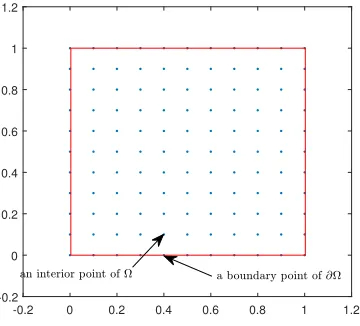
Figure 1. Considered domain Ω of Example4.1.

-0.2 0 0.2 0.4 0.6 0.8 1 1.2 -0.2

0 0.2 0.4 0.6 0.8 1 1.2

Example 4.1. Consider Eq. (1.1) with two sub-examples corresponding to sets of differ-ent parameters ofa= 1, b= 1, c= 0.7 andα, β∈ {10n s.t. n= 3,4,5,6}via various mesh spatial and time stepsh= 0.2, 0.1, 0.05 andδt= 0.01, 0.001 on the domain as Figure 1. The corresponding exact solution of the collective parameters is given by

u1(x, t) =e

−t

sin(πx1) sin(πx2),

wherex= (x1,x2), the functionsf(u) = 2u−1

2uandu◦is obtained using the exact solutions.

Table 1,2 presents−log10(r.l.s.e) comparingh= 0.2, 0.1, 0.05 for different values log10α

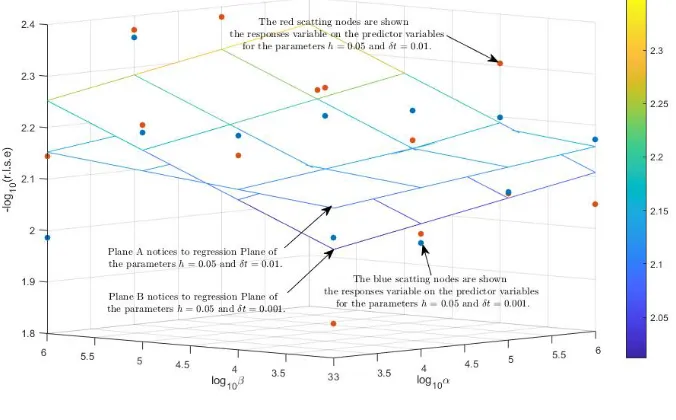
and log₁₀β for δt = 0.01 and 0.001, respectively. In Figure 3, the red and blue points respectively show the dispersion to different values of α and β. Planes A and B are the regression plane based on the spatial common parameter h= 0.05 and the different time parametersδt= 0.01 andδt= 0.001, respectively, which demonstrate growth of the accuracy can be deduced from the growth of the accuracy when increasing auxiliary parametersαand β.

Table 1. Comparing−log₁₀(r.l.s.e) errors forδt= 0.01 of Example4.1 by different parametersα,βandhfor discretization GPS.

h= 0.2 h= 0.1 h= 0.05 log₁₀α= 3 4 5 6 log₁₀α= 3 4 5 6 log₁₀α= 3 4 5 6

Table 2. Comparing−log10(r.l.s.e) errors forδt= 0.001 of Example4.1

by different parametersα,βandhfor discretization GPS.

h= 0.2 h= 0.1 h= 0.05 log10α= 3 4 5 6 log10α= 3 4 5 6 log10α= 3 4 5 6

log10(β) = 3 0.9216 0.9716 0.9025 1.0377 1.5478 1.6951 1.5257 1.5210 1.8673 2.0243 2.0847 2.0473

4 1.0688 1.1887 0.9037 1.0140 1.5052 1.5842 1.7244 1.7792 2.1786 2.2916 2.1720 2.3041 5 1.0522 1.1094 1.1734 1.0364 1.5290 1.5145 1.5334 1.5860 2.2218 2.0915 2.2546 2.1918 6 1.1349 0.9043 1.1242 0.9907 1.5667 1.5021 1.7506 1.7786 2.1441 2.3717 2.3798 2.2610

Figure 2. The above and below planes are estimated by multi-linear regressions of the responses in −log10(r.l.s.e) on the predictors in

log₁₀(α),log₁₀(β)

for the parameters h = 0.05, δt = 0.001 and h = 0.1, δt= 0.01, respectively.

References

[1] K. Atkinson and W. Han,Theoretical numerical analysis, Berlin: Springer, Vol. 39, 2005. [2] H. Brezis,Functional analysis, sobolev spaces and partial differential equations, Springer Science

& Business Media, 2011.

[3] J. J. Duistermaat and J. A. C. Kolk,Distributions, Birkhuser Boston, 2010, 33–44.

[4] V. L. Gertsberg and G. I. Sivashinsky,Large cells in nonlinear Rayleigh-Benard convection, Progress of Theoretical Physics,66(4) (1981), 1219–1229.

[5] N. Hadjisavvas and S. Schaible,Quasimonotone variational inequalities in Banach spaces, Jour-nal of Optimization Theory and Applications,90(1) (1996), 95–111.

[6] M. Ilati and M. Dehghan, Error analysis of a meshless weak form method based on radial point interpolation technique for Sivashinsky equation arising in the alloy solidification problem, Journal of Computational and Applied Mathematics,327(2018), 314–324.

[8] C. S. Liu,Elastoplastic models and oscillators solved by a Lie-group differential algebraic equa-tions method, International Journal of Non-Linear Mechanics,69(2015), 93–108.

[9] R. C. Mittal and S. Dahiya,A quintic B-spline based differential quadrature method for nu-merical solution of Kuramoto-Sivashinsky equation, International Journal of Nonlinear Sciences and Numerical Simulation,18(2) (2017), 103–114.

[10] M. Rouis, and K. Omrani,On the numerical solution of two dimensional model of an alloy solidification problem, Modeling and Numerical Simulation of Material Science,6(01) (2016), 1–9.

[11] W. Rudin,Functional analysis, Internat. Ser. Pure Appl. Math., 1991.

[12] G. I. Sivashinsky,On cellular instability in the solidification of a dilute binary alloy, Physica D: Nonlinear Phenomena,8(1-2) (1983), 243–248.