Statistical data mining for Sina Weibo, a Chinese micro blog: sentiment modelling and randomness reduction for topic modelling

(1)

Micro-blog: Sentiment Modelling and Randomness

Reduction for Topic Modelling

London School of Economics and Political Sciences

Wenqian Cheng

A thesis submitted to the Department of Statistics of the London

School of Economics for the degree of Doctor of Philosophy,

(2)

(3)

I certify that the thesis I have presented for examination for the MPhil/PhD degree of the London School of Economics and Political Science is solely my own work other than where I have clearly indicated that it is the work of others (in which case the extent of any work carried out jointly by me and any other person is clearly identified in it). The copyright of this thesis rests with the author. Quotation from it is permitted, provided that full acknowledgement is made. This thesis may not be reproduced without my prior written consent.

I warrant that this authorisation does not, to the best of my belief, infringe the rights of any third party.

I declare that my thesis consists of approximately 50,000 words.

(4)

Abstract

Before the arrival of modern information and communication technology, it was not easy to capture people’s thoughts and sentiments; however, the development of statistical data mining techniques and the prevalence of mass social media provide opportunities to capture those trends. Among all types of social media, micro-blogs make use of the word limit of 140 characters to force users to get straight to the point, thus making the posts brief but content-rich resources for investigation. The data mining object of this thesis is Weibo, the most popular Chinese micro-blog.

In the first part of the thesis, we attempt to perform various exploratory data mining on Weibo. After the literature review of micro-blogs, the initial steps of data collection and data pre-processing are introduced. This is followed by analysis of the time of the posts, analysis between intensity of the post and share price, term frequency and cluster analysis.

Secondly, we conduct time series modelling on the sentiment of Weibo posts. Considering the properties of Weibo sentiment, we mainly adopt the framework of ARMA mean with GARCH type conditional variance to fit the patterns. Other distinct models are also considered for negative sentiment for its complexity. Model selection and validation are introduced to verify the fitted models.

Thirdly, Latent Dirichlet Allocation (LDA) is explained in depth as a way to discover topics from large sets of textual data. The major contribution is creating a Randomness Reduction Algorithm applied to post-process the output of topic

(5)

(6)

Acknowledgements

First, I would like to express my sincere gratitude to Prof. Piotr Fryzlewicz for the continuous support of my PhD study, for his patience, motivation, and immense knowledge. I am grateful to him for his constructive criticism during my thesis writing and for his encouragement at all stages of my research. This work would not have been done without his continued guidance and generous support. My thanks also goes to Dr. Clifford Lam and Dr. Wicher Bergsma for their comments and suggestions on my work.

I would like to thank the Centre of Analysis of Time Series (CATS) and the Time Series Group of the Statistics Department at LSE for providing a perfect environment in which to pursue research. I am thankful to Ian Marshall (the Research Administrator of the Department of Statistics), and Lyn Grove and Jill Beattie (the Administrators at CATS) for their kind support.

There are many people whose suggestions, discussions and comments have greatly contributed to my PhD work. I very much appreciate Christopher Sciberras’s efforts and kind assistance in proofreading this thesis and correcting my grammatical errors. I am grateful to Dr. Alan Pryor, my master project supervisor, to keep giving me valuable advice and inspiration in my research. I am also grateful to Ivan Sanchez, Dr. Sebastian Riedel and Dr. Nikos Aletras from the Computer Science Department at University College London and Dr. Georg Hahn from the Statistics Department at Imperial College for their comments and suggestions about my research. Hearty thanks go to my colleagues over the years for their stimulating

(7)

discussions and after-work chats. They include Rafal Baranowski, Anna Louise Schroeder, Na Huang, Majeed Simaan, Ewelina Sienkiewicz, Ali Habibnia, Cheng Qian, Yajing Zhu, and Hyeyoung Maeng.

I would also like to extend thanks to the following for their constant and unfailing support, and I could not have managed it without them: Chen Lu, Si Qiao, Ying Chen, Ruoxi Li, Anran Chen, Kun Wang, Jiang Shu, Nawal Mustafa, Michelle Warbis and Cynthia Endezoumou.

Finally, I am very grateful to my family who offered me both spiritual encouragement and financial support throughout all the stages of my research. Thanks for your unconditional love and belief in me.

(8)

Appendix

200

(11)

A.1 Capturing Data via API . . . 200

A.2 Details for Web Crawling . . . 202

A.3 Details for Web Parsing . . . 202

A.4 Additional Results for the Analysis of the Time of the Posts . . . . 204

A.5 Result of Linear Regression for Vanke . . . 207

A.6 Additional Results for Intensity of the Posts vs Share Price . . . 209

A.6.1 Time Series Figures for Company Guomei . . . 209

A.6.2 Time Series Figures for Company Donghang . . . 213

A.6.3 Time Series Figures for Company Biyadi . . . 217

A.7 Word Cloud . . . 221

A.8 Additional Figures for Cluster Analysis . . . 222

B Appendix for Chapter 3 229 B.1 Additional Figures for Positive/Negative Polarity . . . 229

B.2 Additional Figures for Seven Dimensions Sentiments . . . 233

B.3 Details for Fitting Proportional Negative Sentiment Time Series . . 236

(12)

C Appendix for Chapter 4 239

(13)

2.3.1 Daily post amount of Vanke, coloured by time, from 3rd May to 9th Dec 2013. . . 38 2.3.2 Hourly post amount of Vanke. . . 40 2.3.3 Hourly time series plot for Vanke post amount from 3rd May to 9th

December 2013. . . 42 2.3.4 Hourly time series plot for post amount (multiple companies) from

3rd May to 9th December 2013. . . 43 2.4.1 Post amount vs share price for Vanke. . . 45 2.4.2 Dot plot of post amount (x-axis) and share price (y-axis) for Vanke. 46 2.4.3 Time series for share price of Vanke. . . 48 2.4.4 Time series for post amount of Vanke. . . 49 2.4.5 Nadaraya-Watson kernel regression estimate with Bandwith 0.5 for

Vanke (Rt and D0t). . . 51

2.4.6 Regression estimate using local polynomials with Bandwith 0.5 for Vanke (Rt and D0t). . . 52

2.4.7 SiZer plot for Vanke (Rt and Dt0). . . 53

2.6.1 Term frequency for Vanke. . . 58

(14)

2.6.2 Term frequency for Biguiyuan. . . 58

2.6.3 Term frequency for sampled Suning. . . 59

2.6.4 Term frequency for Guomei. . . 60

2.6.5 Term frequency for Donghang. . . 61

2.6.6 Term frequency for Biyadi. . . 61

2.6.7 Term frequency for Maotai. . . 62

2.7.1 Cluster plot from k-means. . . 65

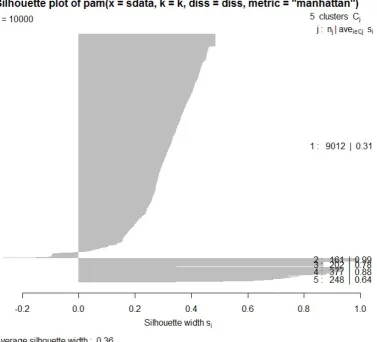
2.7.2 Cluster plot from PAM. . . 68

2.7.3 Silhouette plot for PAM. . . 69

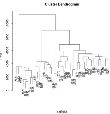
2.7.4 Agglomerative hierarchical clustering. . . 71

3.1.1 Sentiment polarity for company Biyadi using 3 months’ data. . . . 80

3.1.2 3D plot of positive and negative sentiments. . . 81

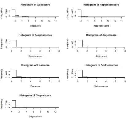
3.1.3 Histograms for seven sentiment dimensions. . . 82

3.1.4 Plots of Good score vs all other scores. . . 83

3.2.1 Original time series for sentiments (top to bottom: Positive, Negative, Overall). . . 86

3.2.2 Proportional time series for sentiments (top to bottom: Positive, Negative, Overall). . . 87

(15)

3.3.2 ACF and PACF plots for proportional positive sentiment time series. 98 3.3.3 Residual plots of AR(1) for proportional positive sentiment time

series. . . 99 3.3.4 QQ plot against normal of AR(1) + ARCH(1) for proportional

positive sentiment time series. . . 102 3.3.5 QQ plot against t-distribution of AR(1) + ARCH(1) for proportional

positive sentiment time series. . . 102 3.3.6 Time series plot for proportional negative sentiment. . . 104 3.3.7 Time series plot for proportional negative sentiment (adjusting the

huge spike between Day 206 and Day 208 by exponential smoothing).104 3.3.8 ACF and PACF plots for proportional positive sentiment time series

(adjusting the huge spike between Day 206 and Day 208 by exponential smoothing). . . 105 3.3.9 Diagnostics plots of Model 1 for proportional negative sentiment

time series. . . 108 3.3.10 Plots of series with 2 conditional standard deviation superimposed

for proportional negative sentiment time series (Top: Model 1 vs Bottom: Model 2). . . 110 3.3.11 QQ plots against skewed normal for proportional negative sentiment

(16)

3.3.12 Time series plot for proportional negative sentiment (adjusting the huge spike between Day 206 and Day 208 by threshold clearance). 113 3.3.13 ACF and PACF plots for proportional negative sentiment (adjusting

the huge spike between Day 206 and Day 208 by threshold clearance).114 3.3.14 QQ plot against skewed t-distribution of Model A for proportional

negative sentiment (adjusting the huge spike between Day 206 and

Day 208 by threshold clearance). . . 115

3.3.15 Comparison of MAE among Model 1, Model 2, and exponential smoothing prediction. . . 120

3.3.16 Comparison of MAE among Model A, Model B, and exponential smoothing prediction. . . 121

3.4.1 Cross-correlation plot for transformed proportional positive and negative sentiment time series. . . 123

3.4.2 Residual plot for VAR model. . . 125

3.4.3 ACF for the residuals of VAR model. . . 126

3.4.4 PACF for the residuals of VAR model. . . 126

4.2.1 Bayesian network of LDA. . . 140

(17)

A.4.1 Daily post amount, coloured by time (Multiple companies: Biguiyuan,

Biyadi, Maotai, Donghang, Guomei, and Suning). . . 205

A.4.2 Hourly post amount (Multiple companies: Biguiyuan, Biyadi, Maotai, Donghang, Guomei, and Suning). . . 206

A.5.1 Dot plot for log returns of share price and log returns of post amount of Vanke. Group A: Rt vs Dt0; Group B: R 0 t vs Dt. . . 207

A.5.2 Result of linear regression for Vanke (Group A: Rt and D0t). . . 207

A.5.3 Result of linear regression for Vanke (Group B: R0_t and Dt). . . 208

A.6.1 Time series for share price of Guomei. . . 209

A.6.2 Time series for post amount of Guomei. . . 210

A.6.3 Regression estimate using local polynomials with Bandwith 0.5 for Guomei (Rt and Dt0). . . 211

A.6.4 SiZer plot for the first derivative for Guomei (Rt and D0t). . . 212

A.6.5 Time series for share price of Donghang. . . 213

A.6.6 Time series for post amount of Donghang. . . 214

A.6.7 Regression estimate using local polynomials with Bandwith 0.5 for Donghang (Rt and D0t). . . 215

A.6.8 SiZer plot for the first derivative for Donghang (Rt and Dt0). . . 216

A.6.9 Time series for share price of Biyadi. . . 217

(18)

A.6.11 Regression estimate using local polynomials with Bandwith 0.5 for

Biyadi (Rt and Dt0). . . 219

A.6.12 SiZer plot for the first derivative for Biyadi (Rt and D0t). . . 220

A.7.1 Word cloud for Biyadi. . . 221

A.8.1 Cluster plot from CLARA. . . 222

A.8.2 Silhouette plot for CLARA. . . 223

A.8.3 Cluster plot from PAM. Sparsity = 0.96. . . 224

A.8.4 Silhouette plot for PAM. Sparsity = 0.96. . . 225

A.8.5 Cluster plot from PAM. Sparsity = 0.95. . . 226

A.8.6 Silhouette plot for PAM. Sparsity = 0.95. . . 227

A.8.7 Agglomerative hierarchical clustering. Sparsity = 0.97. . . 228

B.1.1 Histograms of polarities (comparison between Chinese Emotional Words Ontology (top) and Hownet Chinese Message Structure Base (bottom)). . . 229

B.1.2 Skewness test of positive and negative sentiments. . . 230

B.1.3 Poisson and Negative Binomial distribution fitting. . . 230

B.1.4 Information of Poisson and Negative Binomial distribution fitting. 231 B.1.5 Correlation test of positive and negative sentiments. . . 231

(19)

B.1.7 Top 50 negative sentiment words. . . 232

B.2.1 Scores of seven dimension sentiments. . . 233

B.2.2 Correlation and p-values between different sentiments. . . 234

B.2.3 Plots of Happiness, Surprise score vs other remaining scores. . . 235

B.2.4 Plots of Anger, Fear, Sadness score vs other remaining scores. . . . 235

B.3.1 QQ plot against normal ARMA for proportional negative sentiment (adjusting the huge spike between Day 206 and Day 208 by threshold clearance). . . 238

C.1.1 Example Two: topic words and original posts. . . 240

(20)

List of Tables

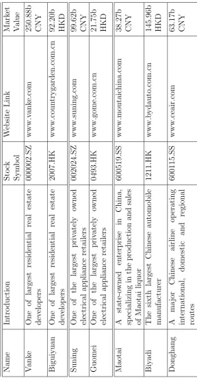
2.1 Descriptions about the companies. . . 34

2.2 Post amount for each company. . . 35

2.3 Stationarity test results . . . 50

2.4 Structure of a term-document matrix . . . 63

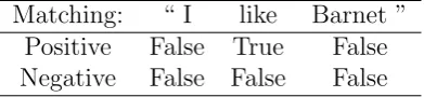
3.1 Example of lexicon-based sentiment matching . . . 76

3.2 Proportional sentiment time series stationarity test results . . . 88

4.1 Randomness Reduction empirical example for the best final intersections at the topic level. . . 165

4.2 Improvement by Randomness Reduction for the first month (3rd May to 2nd June) . . . 170

4.3 Improvement by Randomness Reduction for the second month (2nd Jun to 1st Jul). . . 170

4.4 Improvement by Randomness Reduction for the third month (1st Jul to 1st Aug). . . 171

4.5 Improvement by Randomness Reduction for the fourth month (1st Aug to 1st Sep). . . 171

(21)

4.6 Improvement by Randomness Reduction for the fifth month (1st Sep

to 1st Oct). . . 171

4.7 Improvement by Randomness Reduction for the sixth month (1st Oct to 1st Nov). . . 172

4.8 Improvement by Randomness Reduction for the seventh month (1st Oct to 1st Nov). . . 172

4.9 Summary of results for Randomness Reduction. . . 172

4.10 Summary of results for Randomness Reduction on Twitter data set about Apple . . . 175

4.11 Summary of results for Randomness Reduction on Twitter dataset about US Airlines . . . 177

4.12 Summary of topic categories. . . 179

4.13 Monthly topic evolutions with overlapped periods. . . 180

4.14 Monthly topic evolutions without overlapped periods (Part1). . . . 181

4.15 Monthly topic evolutions without overlapped periods (Part2). . . . 181

4.16 Summary of topic categories by month and by week. . . 182

4.17 Weekly topic evolutions (part1). . . 184

(22)

(23)

Introduction

Social Media is a type of Internet-based application which allows the creation and exchange of user-generated content. It was built on the ideological and technological foundations of Web 2.0 (Oreilly, 2005), which allows users to update status and interact with each other, rather than just retrieve information. Due to the easy accessibility and multimedia nature of microblogging platforms, recently some Internet users tend to migrate from traditional communication applications, such as blogs or mailing lists, to microblogging services.

Authors of those posts broadcast their current status to the public or a selected circle of contacts, discuss current issues and share opinions on a variety of topics. Individuals can also embed shortened URLs, insert hash tags, and comment on others’ posts. The 140 characters word limit of microblogs forces users to get straight to the point, which makes the posts brief but content-rich resources for investigation.

“Weibo” is the Chinese word for “microblog”. Sina Weibo is a Chinese microblogging website which is used by well over 30% of Internet users in China, with a market penetration similar to Twitter in the United States (Rapoza, 2011). Forbidding the usage of Twitter in China resulted in the birth and popularity

(24)

of indigenous Weibo. It was launched by Sina Corporation on 14 August 2009, and attracted 503 million registered users by 2012 (Ong, 2013). Statistics showed there were 100 million daily users on Sina Weibo by the third quarter of 2015 (China-Resonance, 2011).

On average 600 million tweets were generated per day (500 million for twitter (TwitterInc., 2013), 100 million for Weibo (SinaCorp., 2013)), which create extensive resources for statistical data mining. The emotions and attitudes exhibited by these massive user-generated contents would be good indicators for people’s thinking and future behaviours. Researchers, marketeers and political activists see these data as a good source for opinion mining, topic extraction and sentiment analysis for marketing or social studies. How to recognise the valuable parts of those enormous data and carry out statistical studies has become a significant research issue. The information from microblog posts is stored in unstructured formats (text) and not organised using any automated system, resulting in the complexity of data preprocessing and the difficulties of applying statistical methods.

In the literature, Weibo-related research mainly focuses on numerous qualitative analyses for popularity, social effect or verification mechanism, but only a few quantitative analyses could be found, which will be introduced in Section 2.1. My thesis will focus on the Sina Weibo, which is an emerging, attractive and still partially untapped research field. In addition, the research of Weibo sentiment time series modelling and topic modelling is relatively new and there remains much to be explored.

(25)

mining. It starts with a literature review for microblogs and describes how to generate data from Weibo for seven specific companies in Chart 2.1. Before capturing textual features, we conduct quantitative analysis on the pattern of the time of the posts for those specific companies and their relationship with share prices. In the second half of Chapter 2, after introducing Chinese word segmentation, we generated several results from initial text analysis. The term frequency chart can be a good show case for the most important terms and helps to build a basic understanding of the posting content. Clustering methods, such as k-means and k-mediods, are applied to group the posts.

In Chapter 3, we describe some fundamental methods for sentiment analysis and present time series for both positive and negative sentiments. A general framework for univariate time series model fitting is provided in detail, and this framework is then employed for our sentiment time series fitting. Results show that the proportional positive time series fits well using the general framework, while we need alternative approaches to fit the proportional negative time series. Model comparison and validation are presented for proportional negative sentiment after attempting multiple approaches for model fitting. Multivariate time series models are adopted as we intend to model and explain the interactions and comovements between positive and negative sentiment time series. Interesting results are obtained by exploiting the vector autoregressive (VAR) and BEKK models for the Box-Cox transformed time series data.

(26)

(2003). The thorough generative process and model learning using Gibbs sampling are introduced in detail. After applying LDA on our microblog’s data, it can be found that the generated topics contain some randomness. We intend to reduce the randomness and retain stable and well-explained topics for topic evolution analysis. Thus, the Randomness Reduction algorithm for filtering out the insignificant topics and utilising topic distributions to find out the most persistent topics is proposed. Case studies are presented to show the significance of the performance of the algorithm. The filtered topics are then classified and the evolution of these topics is detailed.

(27)

Exploratory Data Mining

2.1

Literature

Review

of

Data

Analysis

of

Microblogs

Before performing initial data analysis and further data mining on Weibo’s data, a requisite is to conduct a literature review to explore previous researches on microblogs. Due to the wider spread and earlier establishment of Twitter, a more considerable body of research can be found on Twitter than on Weibo. The first step is to investigate the relevant literature on Twitter.

2.1.1

Review of Relevant Twitter Data Analysis

There have been several papers on exploring hotspots and examining the predictive power of Twitter. Using Twitter’s data as predictors, researchers illustrated that it is possible to improve the prediction outcomes of disease outbreaks (Louis and Zorlu, 2012), including seasonal influenza (Achrekar et al., 2012). Singh et al. (2012) pointed out that tweets can be used to visualise immediate traffic conditions in London. Improving voting behavior prediction by adding Twitter information

(28)

(Chrzanowski and Levick, 2012), such as elections prediction (Gayo-Avello, 2012a; Chung and Mustafaraj, 2011), is another interesting research topic. However, some counter-views (Gayo-Avello, 2012b) have been put forward against using tweets as a predictive indicator for election. Other studies such as movie performance prediction (Asur and Huberman, 2010) and Oscar prediction (Thelwall et al., 2011) may also be of interest.

There are a few analyses about stock price prediction (Logunov, 2011; Mittal and Goel; Bollen et al., 2011). How the posts from microblogs relate to the fluctuation of stock price is an appealing topic for researchers, and there are many papers on this theme. Most stock prediction practice is based on a large amount of tweets and aims at predicting benchmark stock market indices, rather than focusing on specific companies. One of the most influential papers was by Bollen et al. (2011), investigating whether the measurement of collective mood states generated from large-scale Twitter posts are correlated to the value of the Dow Jones Industrial Average (DJIA), and the results indicate that the accuracy of DJIA predictions was improved significantly by including specific public mood dimensions. In addition, most articles with keywords “microblog” (“Twitter”) and “stock price” also include “sentiment” in their title. This fact implies that sentiment time series modelling is a crucial element for predicting future stock price using microblog posts.

(29)

identifications for English texts, and it was applied by Bollen et al. (2011) and Ramon (2012) for sentiment analysis in their research. We adopted several Chinese lexicons in our research and they will be introduced in Chapter 3. Machine learning algorithms, such as naive Bayes classifier, Support Vector Machine (SVM) and Neutral Networks (NN), were employed as supervised learning methods for sentiment classification in many studies (Xie et al., 2012; Ramon, 2012; Ding et al., 2011; Tian and Zheng, 2012). Supervised learning algorithms examine the training data and develop an inferred function, which can be used for mapping new data. The relevance and quality of training data is crucial when high accuracy is required. However, due to the lack of relevant training data and the difficulties of manually tagging, we will narrow down our sentiment classification to lexicon-based approaches in this thesis.

(30)

regression models were applied for selecting and analysing the content of tweets. To assess the model adequacy, non-linearity and causality tests on the time series were conducted. Results showed that adding the additional time series from Twitter results in an increase in prediction accuracy of 5 percent or more. These studies are closely connected with the research detecting the potential relationship between Weibo’s post amount and share price, which can be a starting point for our Weibo data analysis.

2.1.2

Review of Weibo Data Analysis

According to iResearch’s report (China-Resonance, 2011), Sina Weibo had 56.5% of China’s microblogging market based on active users, and 86.6% based on browsing time over competitors such as Tencent Weibo and Baidu’s services. It successfully went public on Nasdaq under the symbol “WB” in 2014.

(31)

There is little literature in English on Weibo, therefore, we searched for Weibo literature using an official Chinese Academic Platform named China Knowledge Resource Integrated Database (CNKI, 2016). Most papers about Weibo are qualitative analyses, for example about Weibo’s propagation characteristics, posters’ motive and behaviour, and the relationship between Weibo and marketing. Only a few studies have included quantitative analyses on Weibo and these studies will be introduced in the following paragraphs. Reviews will include three main aspects: stock market prediction, hotspot detection, and topic or social affair trend forecasting.

A group of researchers at Shanghai University (Zhou et al., 2013) found that investors’ emotions could be detected from the heat of some keywords on microblogs and could be used to predict stock market fluctuations, which is similar to Twitter analysis for stock price prediction. They defined six keywords which could be translated as “Bull Market”, “Positive News”, “Stock Index rise”, “Bear Market”, “Negative News”, and “Stock Index drop”. The heat of the keywords was defined as the daily number of posts containing those words. The input data were the sequences of the heat and the output data were the fluctuation labels (+1 and -1) of the closing price. A significant Granger causality relationship between “rise” or “drop” and closing prices was found. Results showed that the heat of keywords’ indicated the trend of some events indirectly, and the accuracy was about 59% for “stock index rise” and 78% for “stock index drop”. By setting a lag of one week’s time, the change of heat of these two words could correctly predict the change of Shanghai Composite index in most cases.

(32)

possible hotspots of a certain subject using Weibo data. A case study to find the potential hotspots of the specific field of “data mining” was conducted and compared with other traditional hotspots detecting methods. Sheng (2012) performed word frequency counts, co-word analysis, and social media analysis to find out the hot keywords and academic leaders for this subject, and track them continuously. Comparing those automatically detected hotspot results from Weibo with the topics on Web of Science for “data mining” subject, they found around 30 percent of specific topics were identical. Results showed that making use of Weibo data would improve the hotspot detection further as it could include several more latest hotspots than traditional methods.

Zheng et al. (2012) have proposed an approach for news topics detection using Weibo data. By finding the emerging keywords from a large amount of posts and then clustering them, news topics could be recognised and recorded. To identify the keywords, researchers introduced the compound weight to combine the word frequency and the growth trend. A measurement of the likelihood of a word to be a news keyword was taken, and a contextual relevance model was used to support incremental clustering and construct the topic. The results proved the effectiveness of the approach to detect news topics out of massive messages (3 million posts for 10 days).

(33)

and illustrated fully later in Chapter 4. By calculating aggregation and separation between the short-period and long-period moving average line, breaking events can be recognised. The LDA algorithm is applied to figure out the event-related “word bag” and corresponding weight for the event. The data of the first seven days were used as the training materials and the eighth day’s posts were used to check the prediction. The results of the prediction showed some significance, but the limitation was that only a single case study with small data size and very short time span was conducted.

After reviewing the relevant literature for both Twitter and Weibo, we start our research with some exploratory data mining, such as the time of the posts, the relationship between post amount and share price, term frequency and cluster analysis. Time series modelling on sentiment and topic modelling for hotspots detection will be carried out and clarified in the following chapters.

2.2

Data Collection

(34)

but it is still possible to download posts by individual users or geolocation. The technical details of obtaining data via API can be found in Appendix A.1.

Unlike Web Crawling, specified in Appendix A.2, which downloads all the information from each page, Web Parsing is generally targeted at capturing specific information and transforming unstructured data into structured data that can be stored and analysed in a database. Extensible Markup Language (XML) is adopted for Web Parsing as a markup language that defines a set of rules for encoding data in a format that is both human-readable and machine-readable. The advantage of this method is that there is no need to consider API limits. The disadvantage is that it is still an unofficial method to capture data, so the web page format or the download limit may change. This method had been adopted and kept stable for more than a half year until Sina changed the version of the web interface December in 2013 and included the Captcha to avoid data acquisition from external applications.

(35)

period, and if we intend to capture all of them, the time interval of running our code needs to be relatively short. Thus, due to the limit of the search frequency, we may only choose moderately hot keywords in order to capture continuous data. For instance, if we chose “Baidu” (the most popular Chinese search engine) as our keyword, the number of posts containing “Baidu” will far exceed the limit of 1600 per hour. Thus, we cannot capture a complete dataset for a very popular keyword. In contrast, if a brand is not popular at all, only a few posts can be found within an hour. It will be difficult to conduct text mining or time series analysis.

(36)

[image:36.595.137.426.121.676.2]

(37)

Our data set covers approximately six months and the post amount of each company are listed in Chart 2.2. In summary, the data collection for four companies, Biyadi, Guomei, Donghang and Vanke, started on 3rd May 2013, and for three other companies, Biguiyuan, Maotai and Suning, started on 8th May 2013. Our data collection ended on 9th December 2013 when Sina added Captcha to its login mechanism. More technical details can be found in Appendix A.3.

Table 2.2: Post amount for each company. Company Length Post Amount

Vanke 221 days 247373 Biguiyuan 215 days 94809

Suning 215 days 732684 Guomei 221 days 327298 Maotai 215 days 183539 Biyadi 221 days 134530 Donghang 221 days 38963

(38)

imputation treats the imputed data points as an equal to the original ones, which may cause misleading results (Rubin, 1988). There are on average three gaps in our dataset for each company and the gaps are mostly shorter than one day, so we employed simple imputation: the average of the day before and the day after is calculated as the modified daily post amount. For instance, in Vanke’s data, the post amount on 26th June was only 56, which is unusual, and the average of the 25th and 27th’s amount 1₂(1079 + 1526) = 1303 is used instead. Other methods such as exponential smoothing are employed for missing data and extreme values in Chapter 3 for further sentiment time series modelling.

Apart from some analyses conducted on all the companies, the majority of the analyses in this thesis are mainly based on Vanke’s data. This is due to the fact that, compare to other companies, it has higher quality and a moderate quantity of data. Suning and Guomei include a large number of promoted posts and thus have many bursts and a very large quantity of data. The other companies are less popular than Vanke and have a smaller quantity of data.

2.3

Analysis of the Time of the Posts

In this section, we will investigate the posting patterns by analysing the time of the posts. A series of charts and graphs are created to show the different characteristics of posting time. Most of the analyses in this section are based on the data collected for company Vanke from the start of May till the start of December. The results for the other companies can be found in Appendix A.4.

(39)

Figure 2.3.1 for Vanke and Figure A.4.1 for all the other companies. It seems that the daily number of posts for Vanke during these 7 months are relatively stable at around 1300 posts per day with a slight downward trend, except for three extreme peaks and two gaps of missing data.

By observing the posts over the periods of peaks, we can find possible causes of those extreme peaks. Two peaks around 4th July and 25th November seem to result from breaking news of Vanke. The former appears to be from a news story announcing Vanke ranked as the top 1 in sales value in the “Top 50 ranking in China’s real estate business sales in the first half of 2013”. The latter appears to be due to a news story stating that Vanke evaded land value added tax amounting to 3.8 trillion Yuan. Many Weibo users forwarded and commented on these news, and there were many discussions and follow-ups. The reason for the peak around 29th July is hard to determine. It might result from many promotions and advertisements held by Vanke’s official account during that week. It involved users by drawing prizes from all the forwarders, i.e. the official account will make posts for promotion purpose, and many followers will forward the posts to take the opportunities for random lucky draws, which boosted the post amount and attracted many followers.

(40)

0 1000 2000 3000

5th May 5th Jun 5th Jul 5th Aug 5th Sep 5th Oct 5th Now 5th Dec

Date: from 3rd May to 9th Dec

P

ost Amount

factor(Hour)

0

1

2

3

4

5

6

7

8

9

10

11

12

13

14

15

16

17

18

19

20

21

22

23

[image:40.595.124.501.154.555.2]

Daily Post Amount of Vanke, coloured by Time

(41)

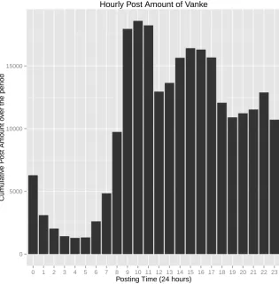
peaks: morning around 10am, afternoon around 3pm, and evening around 10pm. After observing the original posts, the afternoon peak for Suning can be explained as the promotions by Suning were mostly announced on its official account in the afternoon and they initiated many reposts.

The evening peak could indicate that Weibo users talked about Donghang, Maotai, Suning and Guomei more often at home in the evening as they are brands more related to daily life. It may be because airlines (Donghang), liquor (Maotai), and electrical appliances (Suning and Guomei) are more likely to be topics of interest after work than real estate brands (Vanke, Biguiyuan) and automobile brands (Biyadi). These findings are supported by research which focuses on using tweets as an electronic word of mouth (Jansen et al., 2009). Jansen selected brands and categories under the assumption that these brands would be most likely mentioned in and affected by microblogging and after exploring several lists including American Customer Satisfaction Index, Business Weeks Top Brand 100, etc. The categories were chosen to be closely related with items in daily life, which included transportation, food and consumer electronics. Jansen’s findings provide support to the empirical findings described above: Donghang (transportation), Maotai (food), Suning and Guomei (consumer electronics) are in Jansen’s chosen categories and closely linked to daily life.

(42)

0 5000 10000 15000

0 1 2 3 4 5 6 7 8 9 10 11 12 13 14 15 16 17 18 19 20 21 22 23

Posting Time (24 hours)

Cum

ulativ

e P

ost Amount o

v

er the per

iod

[image:42.595.164.480.226.547.2]

Hourly Post Amount of Vanke

(43)

(44)

Hourly Time Series Plot for Vanke Post Amount

Time by Hours (from 3rd May to 9th Dec)

Hour

ly P

ost Amount

0

1000

2000

3000

4000

5000

0

100

200

300

400

[image:44.595.113.512.178.576.2]

500

(45)

(46)

2.4

Intensity of Posts vs Share Price

After analysing only the time of the posts, we are interested in the relationship between the intensity of posts of a company and this company’s share price. In this section, we will focus on Vanke to analyse the potential relationship. The historical daily adjusted closing prices (adjusted for dividends and splits) of Vanke (Symbol: 000002.SZ) between 3rd May and 9th December are downloaded from the Yahoo!Finance (2016) website and recorded as original share prices.

We denote the post amount at dayt asAt and the original share price at day t as

Pt. Initially, a line chart combiningAt andPt is drawn in Figure 2.4.1. There seem

to be some similar patterns between share price and post amount at the beginning of the period. A dot plot forAt and Pt for Vanke is produced in Figure 2.4.2, and

a weak correlation between the post amount and share price according to the plot can be seen. We conduct several tests in this section to further investigate the relationship.

One of the difficulties of processing the time series is dealing with the weekend gaps in share price. First, we create two modified time series and make the denotations: Pt: Original Share Price at dayt

P_t0: Modified Share Price at day t (create Saturday’s share price and Sunday’s as Friday’s)

At: Original Post Amount at dayt

(47)

YMD.SP$Date

YMD.SP$Amount

May Jun Jul Aug Sep

0 1000 2000 3000 ● ● ● ● ● ● ● ●● ● ● ● ● ● ● ● ● ● ●● ● ● ●● ● ● ●●● ●● ● ● ● ●● ● ● ● ● ● ● ● ● ● ● ● ● ● ● ●●●● ● ● ● ● ● ● ● ● ● ● ● ● ● ●● ● ● ●● ● ●●● ● ●●● ● ● ●●● ● ● ●● ● 9 10 11 12 YMD.SP$Adj.Close

Posts Amount Share Price

Figure 2.4.1: Post amount vs share price for Vanke. The dotted pink line represents the share price and the blue line represents the post amount. The share price gaps are due to the closure of the stock market during weekends.

Group A (without weekends): Pt vs A0t

Group B (with weekends): P_t0 vs At

(48)

Figure 2.4.2: Dot plot of post amount (x-axis) and share price (y-axis) for Vanke. 1992), the Augmented Dickey-Fuller (ADF) test (Dickey and Fuller, 1979) and the Phillips-Perron (PP) test (Phillips and Perron, 1988) are applied to accomplish this task and validate each other. The KPSS test is a stationarity test with a null hypothesis that an observable time series is stationary around a deterministic trend. It can be used for both level stationarity and trend stationarity. If the result of the p-value is larger than 0.05, it means that H0 can not be rejected, thus

indicating stationarity. However, in the other two tests, the ADF test and the PP test, p-values smaller than 0.05 indicate stationarity.

(49)

the approximation log(1 +r) ≈ r ensures they are close in value to raw returns. Another advantage of looking at the log returns of a series is that the relative changes in the variable can be seen and compared directly with other variables whose values may have very different base values. For the post amount, if we assume that some news and promotions last several days and the transmission and popularity of a brand depend on yesterday’s, we can expect the hotness of today’s keywords based on yesterday’s, then we may still try to calculate log returns for the daily differences.

We denote the log returns of the time series:

Rt: Log Return of Original Share Price (Rt= log(Pt)−log(Pt−1))

R_t0: Log Return of Modified Share Price (R0_t= log(P_t0)−log(P_t0₋₁)) Dt: Log Return of Original Post Amount (Dt= log(At)−log(At−1))

D0_t: Log Return of Modified Post Amount (D_t0 = log(A_t0)−log(A0_t₋₁))

The time series plots which regard the share price and post amount can be found separately in Figure 2.4.3 and 2.4.4. For the share price figure, the first row shows the three time series Pt, log(Pt), Rt for the original share price (no weekends) and

the second row shows the three time series P_t0, log(P_t0), R0_t for the modified time series of share price (Friday’s share price is applied to Saturday’s and Sunday’s). The first row shows the three time series At, log(At), Dt for the original post

amount and the second row shows the three time series A0_t, log(A0_t), D_t0 for the modified post amount (weekend data deleted).

(50)

Figure 2.4.3: Time series for share price of Vanke (First row, from left to right: Pt,

log(Pt), Rt. Second row, from left to right: Pt0, log(Pt0), R0t).

(51)

Figure 2.4.4: Time series for post amount of Vanke (First row, from left to right: At, log(At), Dt. Second row, from left to right: A0t, log(A

0

t),D

0

t).

the dependent variable (y) are built. The outcomes of linear regression for Group A and Group B can be found in Figure A.5.2 and A.5.3 respectively. From the regression model A.5 and results listed in Appendix, it can be concluded that we can hardly find any evidence for the linear relationship between log returns of post amount and share price.

To analyse further the potential relationship between share price and post amount, we introduce kernel smoothing methods (Wand and Jones, 1994) to find smoother lines for the relationship and determine whether they are significantly different from zero or not.

(52)

Table 2.3: Stationarity test results

Case KPSS test ADF test PP test Stationarity Pt 0.01 0.6146 0.5847 non-stationary

log(Pt) 0.01 0.5955 0.5448 non-stationary

Rt 0.1 0.03371 0.01 stationary

R0_t 0.1 0.01 0.01 stationary At 0.1 0.09092 0.01 almost stationary

log(At) 0.04968 0.207 0.01 almost stationary

Dt 0.1 0.01 0.01 stationary

A0_t 0.1 0.03309 0.01 stationary log(A0_t) 0.04968 0.08175 0.01 almost stationary

D0_t 0.1 0.01 0.01 stationary

polynomial regression (Fan et al., 1995) are applied as the kernel smoothers. The bandwidth of a kernel density estimate can be customised or selected using direct plug-in methods. We choose the direct plug-in approach, where the unknown functionals that appear in expressions for the asymptotically optimal bandwidths are replaced by kernel estimates (Ruppert et al., 1995). Both of the kernel methods are applied to Group A: log return of original share price Rt and log return of

modified post amount D0_t.

(53)

SiZer result for the first derivative is shown in Figure 2.4.7. Vanke’s SiZer graph indicates that the derivatives of the smoother line is not significantly different from zero (with most parts purple). That is to say, we can not detect a significant relationship between log returns of share price and post amount for Vanke.

The results for other companies can be found in Appendix A.6, including time series plots for original/modified share price and post amount, plots of their log and log returns, regression estimate using local polynomials, and plots of SiZer. All the results show a limited relationship between share price and post amount.

● ● ● ● ● ● ● ● ● ● ● ● ● ● ● ● ● ● ● ● ● ● ● ● ● ● ● ● ● ● ● ● ● ● ● ● ● ● ● ● ● ● ● ● ● ● ● ● ● ● ● ● ● ● ● ● ● ● ● ● ● ● ● ● ● ● ● ● ● ● ● ● ● ● ● ● ● ● ● ● ● ● ● ● ● ● ● ● ●

−1.0 −0.5 0.0 0.5 1.0

−0.05

0.00

0.05

Log Return of Original Share Price

Log Retur

n of Modified P

ost Amount

(54)

● ● ● ● ● ● ● ● ● ● ● ● ● ● ● ● ● ● ● ● ● ● ● ● ● ● ● ● ● ● ● ● ● ● ● ● ● ● ● ● ● ● ● ● ● ● ● ● ● ● ● ● ● ● ● ● ● ● ● ● ● ● ● ● ● ● ● ● ● ● ● ● ● ● ● ● ● ● ● ● ● ● ● ● ● ● ● ● ●

−1.0 −0.5 0.0 0.5 1.0

−0.05

0.00

0.05

Log Return of Original Share Price

Log Retur

n of Modified P

ost Amount

(55)

−1.0 −0.5 0.0 0.5

−0.4

−0.2

0.0

0.2

0.4

0.6

x$x.grid

lo

g10

(

h

)

Figure 2.4.7: SiZer plot for Vanke (Rt and Dt0). X-axis represents the log returns

(56)

2.5

Chinese Word Segmentation

Initial quantitative and time series analyses provide a brief description of the general patterns for the posts, but they are not sufficient for understanding what people generally posted about these companies. Thus, further textual analysis, as a complement of quantitative methods, would provide insight on the contents that people posted about. This textual analysis can be also referred to as text mining, a process of deriving the patterns and trends from texts through means such as statistical pattern learning. Typical text mining tasks include text categorization, text clustering, concept/entity extraction, sentiment analysis, document summarisation, and entity relation modelling. It is a part of statistical pattern learning, which aims to use artificial intelligence to learn from data. In this and next two sections, we will first introduce Chinese word segmentation and term frequency analysis as basic text mining, and then explore cluster analysis for grouping posts based on their contents. Next chapters will further discuss sentiment modelling and topic modelling. For quantitative data analyses that only research the amount of posts, there are no other steps required for data pre-processing. Nevertheless, when attempting text mining, some additional steps are requisite. Unlike English, which contains spaces between adjacent words, all Chinese characters are written together. Therefore, word segmentation is essential for Chinese text as an extra step before text mining. As the segmentation influences further textual analysis, it is crucial to find a way to segment Chinese sentence accurately and efficiently.

(57)

segmentation. All of them are originally based on Java. The oldest one built on the MMSEG (Tsai, 2000) for Java Lucene Chinese Analyser, is named rmmseg4j. The problem of this method is that the corpus contains many old-fashioned words, making it insufficient to cope with modern microblog texts. The latest version enables the function of inserting a list of words into the corpus, which means one can add new words or new definitions to be used for word segmentation. But it still lacks the ability for detecting and inserting a large amount of new words efficiently. Another package called rsmartcn, separates words by their semantics effectively and at a faster speed. It forms a port to Imdict Chinese Analyser, which applies an authoritative algorism ICTCLAS (Zhang et al., 2003) based on Hidden Markov Model (HMM) designed by the Chinese Academy of Sciences.

The latest Chinese word segmentation tool is Rwordseg (Li, 2012). It uses rJava to call the Java word segmentation tool Ansj (Sun, 2012), which is an improved port based on ICTCLAS. Compared to rsmartcn, it contains some advance functions, such as separating a combination of Chinese and English, adding Part-of-speech tagging, and inserting new external lexicons. We applied this package for Chinese word segmentation in further Weibo text mining.

2.6

Term Frequency

(58)

to create a corpus. In linguistics, a corpus is a large and structured set of texts and can be used to undertake further statistical analysis. We clean up the data by removing punctuation, numbers, links and English letters. A group of Chinese stop words is removed using a wide-spread Chinese stop words list. Several dictionaries are added from the Sogou Word Database (one of the most widely-used Chinese pinyin input method providers) for popular cyberwords and social media buzz words, and a glossary for those specific companies, e.g. the CEO’s name, affiliated brand names, competitor names, etc., is attached. The minimum topic-word length is set as two, in order to ensure the vocabulary for word frequency only contains sensible terms. This is because a single term with a single character in Chinese does not usually imply a well-defined semantic meaning.

A term frequency chart is a data frame containing most frequent terms with their frequencies, generated in a descending order. It is useful to develop a basic understanding of what the public generally mention about the companies. It can also be helpful to check the correctness of word segmentation, attach specific words to the lexicon, and add extra words to the stop words list.

The term frequency charts for our seven companies can be found in Figures 2.6.1, 2.6.2, 2.6.3, 2.6.4, 2.6.5, 2.6.6, and 2.6.7. All the term frequency charts are generated using all the posts that we collected, except Suning, for which we run a random sample of 200,000 posts, due to the large quantity of original dataset (732,684 posts).

(59)

regions and the name of CEO can also be discovered in several charts. We can also find out many promotion-related terms and understand how they promote themselves. The following sections will list some most frequent terms and discuss the information related to these terms.

2.6.1

Most Frequent Terms for Vanke and Biguiyuan

(60)

Figure 2.6.1: Term frequency for Vanke.

Figure 2.6.2: Term frequency for Biguiyuan.

2.6.2

Most Frequent Terms for Suning and Guomei

(61)

both). The most important competitors for both companies is Jingdong, a Chinese electronic commerce company (rank 17 and 16), but not each other. Individuals mentioning Guomei are likely to mention Suning (rank 15), but there are many posts only containing Suning (we cannot find “Guomei” in Suning’s chart). The most popular products for Suning are refrigerator (rank 10), phone (rank 11), and computer (rank 19). It seems that Suning had a promotion on the National day (rank 14) and had a lucky draw for its followers (rank 6, 32 and 34). While for Guomei, the promotion is likely to be for the eighth year anniversary (rank 25), and the membership policy, which is mentioned very frequently (rank 12), might be one of their business strategies.

(62)

Figure 2.6.4: Term frequency for Guomei.

2.6.3

Most Frequent Terms for Donghang, Biyadi and

Maotai

(63)

Figure 2.6.5: Term frequency for Donghang.

(64)

Figure 2.6.7: Term frequency for Maotai.

2.6.4

Beyond Term Frequency

(65)

2.7

Cluster Analysis

A term frequency chart can provide the top keywords that individuals are the most likely to mention for a specific company, but it can hardly group those posts based on their contents addressing different aspects and provide a comprehensive description of what individuals are posting about. Cluster analysis is to group a set of objects in a way such that the objects in the same group (called cluster) are more similar to each other than to those in other clusters. In cluster analysis, we treat each post as an object, and we intend to group the posts based on the key words which they contain.

Table 2.4: Structure of a term-document matrix

Document 1 Document 2 Document 3 Document 4 . . .

Term 1 1 0 1 0 . . .

Term 2 0 1 0 1 . . .

Term 3 1 2 1 0 . . .

Term 4 0 0 1 1 . . .

Term 5 0 1 0 2 . . .

. . . .

(66)

reduced by controlling the sparsity, which will be described later.

Using term-document matrix, we are able to calculate the distances between posts, and then group the posts into different clusters by different clustering methods in a high-dimensional space. The clusters can be visualised in a bivariate or a trivariate plot, in which each post is represented by a point according to principal components or multidimensional scaling. As an example, in Figure 2.7.1 the clusters are visualised by two leading principal components in the two-dimensional space. Three different cluster algorithms are adopted in our research: k-means (Hartigan and Wong, 1979), k-medoids (Kaufman and Rousseeuw, 1990) and hierarchical clustering (Kaufman and Rousseeuw, 1990).

(67)

−15

−10

−5

0

−2

0

2

4

6

CLUSPLOT( MatrixWeiboForCluster )

Component 1

Component 2

These two components explain 78.85 % of the point variability.

● ● ● ● ● ● ● ● ● ● ● ● ● ● ● ● ● ● ● ● ● ● ● ● ● ● ● ● ● ● ● ● ● ● ● ● ● ● ● ● ● ● ● ● ● ● ● ● ● ● ● ● ● ● ● ● ● ● ● ● ● ● ● ● ● ● ● ● ● ● ● ● ● ● ● ● ● ● ● ● ● ● ● ● ● ● ● ● ● ● ● ● ● ● ● ● ● ● ● ● ● ● ● ● ● ● ● ● ● ● ● ● ● ● ● ● ● ● ● ● ● ● ● ● ● ● ● ●

1

2

3

4

5

6

7

8

9

10

11

12

13

14

15

16

17

18

19

20

2122

23

24

25

26

27

28

29

30

31

32

33

34

35

36

37

38

39

40

41

42 43

44

45

46

47

48

49

50

51

52

53

54

55

56

6162

57

58

59

60

63

64

65

66

67

68

69

70

71

72

73

74

75

76

77

78

79

80

81

82

83

84

85

86

87

88

89

90

91

92

93

94

95

96

97

98

99

100

103

101

102

104

105

106

107

108

109

110

111

112

113

114

115

116

117

118

119

120

121

122

123

124

125

126

127

128

129

130

131

132

133

134135

136

137

138

139

140

141

142

143

144

145

146 147

148

149

150 151

152

153

154

155

156

157

158

159

160

161

162

163

164

165

166

167

168

169

170

171

172

173

174

175

176

177

178

179

180

181

182

183

184

185

186

187

188

189

190

191

192

193

194

195

196

197

198

199200

201

202

203

204

205 206

207

208

209

210

211

212

213

214

215

216

217

218

219

220

221

222

223

224

225

226

227

228

229

230

231

232

233

234

235

236

237

238

239

240

241

242

243

244

245 246

247 248

249

250

251

252

253

254

255

256

257

258

259

260

261

262

263

264

265

266

267

268

269

270

271

272

273

274

275

276

277 278

279

280

281

282

283

284

285

286

287288

289

290

291

292

293

294

295

296

297

298

299

300301

302

303

304

305

306

307

308

309

310

311

312

313

314

315

316

317

318

319

320

321

322

323

324

325

326

327 328

329

330

331

332

333

334

335

336

337

338

339

340

341

342

343

344

345

346

347

348

349

350

351

352

353

354

355

356

357

358

359

360

361

362

363

364

365

366

367

368

369

370

371

372

373

374

375

376

377

378

379 380

381

382

383

384

385

386

387

388

389

390

391

392

393

394

395

396

397

399

398

400

401

402

403

404

405

406

407

408

409

410

411

412

413 414

415

416

417

418

419

420

421

422

423

424

425

426

427

428

429

430

431

432

433

434

435

436

437

438

439

440

441

442

443

444

445

446

447

448

449

450

451

452

453

454

455

456

457

458

459

460

461

462

463

464

465

466

467 468

469

470

471

472

473

474

475

476

477

478

479

480

481

482

483

484

485

486

487

488

489

490

491

492

493

494

495

496

497

498

499

500

501

502

503

504

505

506

507

508

509

510

511

512

513

514

515

516

517

518

519

520

521

522

523

524

525

526

527

528

529

530

531

532

533

534

535

536

537

538

540

539

541

542

543

544

545

546

547

548

549

550

551

552

553

554

555

556

557

558

559

560

561

562

563

564

565

566

567

568

569

570

571

572

573

574

575

576

577

578

579580

581

582

583

584

585

586

587

588

589

590

591

592

593

594

595

596

597

598

599

600

601

602

603

604

605

606

607

608

609

610

611

612

613

614

615

616

617

618

619

620

621

622

623

624

625

626

627

628

629

630

631

632

633

634

635

636

637

638

639

640

641

642

643

644

645

646

647

648

649

650

651652

654

653

655

656

657

658

659

660661

662

663

664

665

666

667

668

669

670

671

672

673

674

675

676

677

678

679

680

681

682

683

684

685

686

687 688

689

690

691

692

693

694

695

696

697

698

699

700

701

702

703

704

705

706

707

708

709

710

711

712

713

714

715

716

717

718

719

720

721 722

723

724

725

726

727

728

729

730

731

732

733

734

735

736

737

738

739

740

741

742

743

744

745

746

747

748

749

750

751

752

753

754

755

756

757

758

759

760

761

762

763

764

765

766

767

768

769

770

771

772

773

774

775

776

777

778

779

780

781

782

783

784

785

786

787

788

789

790

791

792

793

794

795

796

797

798

799

800

801

802

803

804

805

806

807

808

809

810

811

812

813

814

815

816

817

818

819

820

821

822

823

824825

826

827

828

829

830

831

832

833834

835

836

837

838

839

840

841

842

843

844

845

846

847

848

849

850

851

852

853

854

855

856

857

858

859

860

861

862

863

864

865

866

867

868

869

870

871

872

873

874

875

876

877

878

879

880

881

882

883

884

885

886

887

888

889

890

891

892

893

894

895

896

897

898

899

900

901

902

903

904

905

906

907

908

909

910

911

912

913

914

915

916

917

918

919

920

921

922

923

924

925

926

927

928

929

930

931

932

933

934

935

936

937

938

939

940

941

942

943

944

945

946

947

948

949

950

951

952

953

954

955

956

957

958

959

960

961

962

963

964

965

966

967

968

969

970

971

972

973

974

975

976

977

978

979

980

981

982

983

984

985

986

987

988

989

990

991

992

993

994

995

996

997

998

999

1000

1001

1002

1003

1004

1005

1006

1007

1008

1009

1010

1011

1012

1013

1014

1015

1016

1017

1018

1019

1020

1021

1022

1023

1024

1025

1026

1027

1028

1029

1030

1031

1032

1033

1034

1035

1036

1037

1038

1039

1040

1041

1042

1043

1044

1045

1046

1047

1048

1049 1050

1051

1052

1053

1054

1055

1056

1057

1058

1059

1060

1061

1062

1063

1064

1065

1066

1067

1068

1069

1070

1071

1072

1073

1074

1075

1076

1077

1078

1079

1080

1081

1082

1083

1084

1085

1086

1087

1088

1089

1090

1091

1092

1093

1094

1095

1096

1097

1098

1099

1100

1101

1102

1103

1104

1105

1106

1107

1108

1109

1110

1111

1112

1113

1114

1115

1116

1117

1118

1119

1120

1121

1122

1123

1124

1125

1126

1127

1128

1129

1130

1131

1132

1133

1134

1135

1136

1137

1138

1139

1140

1141

1142

1143

1144

1145

1146

1147

1148

1149

1150

1151

1152

1153

1156

1154

1155

1157

1158

1159

1160

1161

1162

1163

1164

1165

1166

1167

1168

1169

1170

1171

1172

1173

1174

1175

1176

1177

1179

1184

1178

1180

1181

1182

1183

1185

1186

1187

1188

1189

1190

1191

1192

1193

1194

1195

1196

1197

1198

1199

1200

1201

1202

1203

1204

1205

1206

1207

1208

1209

1210

1211

1212

1213

1214

1215

1216

1217

1218

1219

1220

1221

1222

1223

1224

1225

12261227

1228

1229

1230

1231

1232

1233

1234

1235

1236

1237

1238

1239

1240

1241

1242

1243

12441245

1246

1247

1248

1249

1250

1251

1252

1253

1254

1255

1256

1257

1258

1259

1260

1261

1262

1263

1264

1265

1266

1267

1268

1269

1270

1271

1272

1273

1274

1275

1276

1277

1278

1279

1280

1281

1282

1283

1284

1285

1286

1287

1288

1289

1290

1291

1292

1293

1294

1295

1296

1299

1297

1298

1300

1301

1302

1303

1304

1305

1306

1307

1308

1309

1310

1311

1312

1313

1314

1315

1316

1317

1318

1319

1320

1321

1322

1323

1324

1325

1326

1327

1328

1329

1330

1331

1332

1333

1334

1335

13361337

1338

1339

1340

1341

1342

1343

1344

1345

13461347

1348

1349

1350

13511352

1353

1354

1355

1356

13571358

1359

1360

1361

1362

1363

1364

1365

1366

1367

1368

1369

1370

1371

1372

1373

1374

1375

1376

1377

1378

1379

1380

1381

1382

1383

1384

1385

1386

1387

1388

1389

1390

1391

1392

1397

1393

1394

1395

1396

1398

1399

1400

1401

1402

1403

14041405

1406

1407

1408

1409

14101411

1412

1413

1414

14151416

1417

1420

1425

1418

1419

1421

1422

1423

1424

1426

1427

1428

1429

1430

1431

1432

1433

1434

1435

1436

1437

<

Statistical data mining for Sina Weibo, a Chinese micro blog: sentiment modelling and randomness reduction for topic modelling

Micro-blog: Sentiment Modelling and Randomness

Abstract

Acknowledgements

Contents

Appendix

List of Tables

Introduction

Exploratory Data Mining

Review of Relevant Twitter Data Analysis

Review of Weibo Data Analysis

Data Collection

Analysis of the Time of the Posts

factor(Hour)

Hourly Time Series Plot for Vanke Post Amount

0

0

Chinese Word Segmentation

Term Frequency

Most Frequent Terms for Vanke and Biguiyuan

Most Frequent Terms for Donghang, Biyadi and

0

0

CLUSPLOT( MatrixWeiboForCluster )