Solving a robust capacitated arc routing problem using a hybrid simulated annealing algorithm: A waste collection application

Journal of Industrial Engineering and Management Studies

Vol. 3, No. 1, pp. 61 - 76

www.jiems.icms.ac.ir

Solving a robust capacitated arc routing problem using a hybrid simulated

annealing algorithm: A waste collection application

E. Babaee Tirkolaee1*, M. Alinaghian2, M. Bakhshi Sasi2, M. M. Seyyed Esfahani1

Abstract

The urban waste collection is one of the major municipal activities that involves large expenditures and difficult operational problems. Also, waste collection and disposal have high expenses such as investment cost (i.e. vehicles fleet) and high operational cost (i.e. fuel, maintenance). In fact, making slight improvements in this issue lead to a huge saving in municipal consumption. Some incidents such as altering the pattern of waste collection and abrupt occurrence of events can cause uncertainty in the precise amount of waste easily and consequently, data uncertainty arises. In this paper, a novel mathematical model is developed for robust capacitated arc routing problem (CARP). The objective function of the proposed model aims to minimize the traversed distance according to the demand uncertainty of the edges. To solve the problem, a hybrid metaheuristic algorithm is developed based on a simulated annealing algorithm and a heuristic algorithm. Moreover, the results obtained from the proposed algorithm are compared with the results of exact method in order to evaluate the algorithm efficiency. The results have shown that the performance of the proposed hybrid metaheuristic is acceptable.

Keywords:Waste collection, CARP, hybrid metaheuristic algorithm, simulated annealing algorithm, robust optimization.

Received: Mar2016-09 Revised: Jul 2016-04 Accepted: Nov 2016-25

1.

Introduction

The solid waste production and its corresponding incompatibility (e.g. social, economic and environmental incompatibility) have encountered the management of municipal services with a lot of problems in the field of collection, transportation, processing and disposal of such wastes. Since between 75 and 80 percent of the cost of solid waste material management relates to its collection and transportation (Golden et al. 2001) therefore, evaluation and optimization of this system play a significant role in reducing the municipal services management problems. Waste materials must be collected, transferred and disposed as soon as possible and by complying

* Corresponding Author.

1

Department of Industrial Engineering, Mazandaran University of Science and Technology, Babol, Iran.

hygiene recommendations. So that, the best method is to collect them directly from the houses and then, transport them to the disposal facility. Based on above, the importance of waste collection optimal system becomes more evident than before. As a result, choosing the optimal policy for waste collection has a decisive role in cost reduction.

Anyway, there are several kinds of vehicle routing problem to collect the urban waste. Two main categories of routing problem in waste collection are as follows (Beltrami and Bodin 1974): 1) Node Routing Problem: The problem includes commercial waste collection (e.g. the garbage of restaurants, organizations and etc.) such that there are large containers in the main streets of the city which are loaded by the vehicles. In this problem, the containers are considered as nodes, 2) Arc Routing Problem: The problem includes household waste collection in the network of streets and alleys in the city where the wastes are kept in small shelves or garbage bags. Actually, in this problem, the precise location of each customer is not required.

In the household waste collection, the wastes are along the edges. In addition, the capacities of vehicles are limited and they will decrease when they move from one alley to another one or from one arc to another.

Beltrami, E. and Bodin, L. D. (1974) presented one of the first routing problems for the urban waste collection in the form of classical vehicle routing problem (VRP) in order to collect wastes in New York and Washington Municipalities. The problem included the different types of vehicles (i.e. trucks, trolley boats, tug ships, mechanical vacuums). They were able to improve Clarke and Wright algorithm in determining the optimal route. The outcome of their study was implemented in the municipalities and made high advantages for the cities.

Santos et al. (2010) suggested a modified ant colony algorithm to solve the capacitated arc routing problem (CARP). They made some modifications in the initial population, ant decision rule and local search procedure. Finally, they implemented their algorithm for seven standard sets of available examples in CARP literature and obtained appropriate results.

Fleury and Lacomme (2004, 2005) formulated a stochastic arc routing problem (SCARP) for the first time in which some parameters (customers’ demands, vehicles travel times, etc.) were stochastic. In the waste collection problem, customers’ demands can be random in nature or can be considered as a decision variables.

Laporte et al. (2010) presented a CARP problem considering stochastic demands. In the problem, if the capacity of the vehicles are exceeded, failure will occur in the paths. They solved the problem by a neighborhood search heuristic algorithm.

Chen et al. (2014) presented a CARP to formulate a routing problem for investigating the maintenance activities of a road network. In their problem, traveling and servicing time were stochastic. The model was developed using chance constraint programming and it was solved by a branch and bound algorithm.

Willemse and Joubert (2016) presented a new mathematical model for CARP considering intermediate facilities and time limitation. Furthermore, they developed four heuristics to solve the problem and compared their efficiency. Chen et al. (2016) presented a metaheuristic method (HMA) for CARP. The proposed method was able to solve the problem instances in a reasonable time and improved the solution for 6 classic instances and 9 large size instances. They also investigated the effects of the parameters of the algorithm on the results.

Yu and Lin (2015) developed a metaheuristic for the time-dependent prize-collecting arc routing problem. In their study, objective function is determined by subtracting the route traversing cost from the profit gained from the specific route. Also, the traversing time of the edges depends on the departure time of the vehicles.

hand, these changes will cause uncertainty in the data. Moreover, the occurrence of unexpected incidents and disasters are the other reasons of uncertainty in the parameters of CARP.

The aim of this paper is to present an innovative mathematical model for the robust CARP in regards with the waste collection problem which aims to minimize the total cost (the usage cost of vehicles and traversing cost of the edges) considering the demand uncertainty of the required edges. Also, the number of required vehicles to service the all required edges can be determined by the proposed model.

With regard to the NP-hardness of the problem (Golden and Wong 1981), a hybrid metaheuristic algorithm is presented based on a simulated annealing and a constructive heuristic algorithm to solve the problem. Additionally, this work adopts the concept of Taguchi method into the proposed algorithm to enhance the solution quality.

The remainder of the current paper is organized as follows; in section 2, the robust optimization approach of Bertsimas and Sim is discussed. In section 3, the mathematical model for robust CARP specific to the urban waste collection is presented. In section 4, the proposed solution method for the problem is presented. Finally, in section 5, the experimental results are presented.

2.

Robust CARP

The problem includes determining the optimal number of vehicles and the optimal tours for each vehicle with regard to the objective function which minimizes the usage cost of vehicles and the traversing cost of all traversed edges. In this problem, the vehicles are in the depot, firstly. They begin their tours to service the required edges and then, they return to the depot after filling their capacity. The capacity constraint of vehicles results in determining the number of required vehicles. Moreover, demand is uncertain. Thus, the robust model is presented based on the interval robust optimization approach.

2.1.Problem assumptions

-The objective function, in addition to the minimization of traversing cost of the edges, is to minimize the number of required vehicles to meet the total demand.

-Each required edge is serviced only by one vehicle. Also, only one depot is considered in the problem.

- The vehicles are homogeneous and the graph network is asymmetric. Each vehicle begins the tour from the depot and returns there finally.

- The traversing time and the cost of routes are the same among the vehicles.

- The demand of required edges fluctuates in the uncertainty interval d_ij d_ij,d_ij d_ij

 

 _{ } 

 

 .

2.2.Sets, parameters and variables

In this section, the robust model of the proposed problem is presented. For this purpose, sets, parameters and variables are defined firstly. Then, the theoretical basis of the robust optimization is described and finally, the robust model is presented.

Sets

V : Set of the nodes

K : Set of the vehicles

n : Set of the available nodes in the graph network

E : Set of all the edges defined in the network

R

E : Set of all the required edges defined in the network

[ ]

V S : Set of the nodes defined in S

Parameters

ij

c : Traversing cost of the edge( , )i j , such that ( , )i j E

ij

d : Demand of edge( , )i j , such that ( , )i j E

k

cv : Cost of kth vehicle usage

W : Vehicle capacity

M : A very large number

Decisionvariables

xijk: 1 if edge ( , )i j E is traversed by vehicle k, otherwise 0.

yijk: 1 if edge ( , )i j E is serviced by vehicle k, otherwise 0.

uk: 1 if vehicle k is being used such that kK , otherwise 0.

2.3.The robustness of capacity constraints of vehicles

In this section, a robust mathematical model for the classic arc routing problem is formulated based on Bertsimas and Sim approach (2003, 2004). In this model, the uncertain parameter d_ij

takes value in a symmetric interval d_ij d_ij,d_ij d_ij

 

 _{ } 

 

 , where dij



is the deviation ofd_ij. This

parameter causes uncertainty in the capacity constraints of vehicles. The corresponding constraints with uncertainty are:

(1)  ,

,

R

ij ijk i j E

d y W k K



  



So, the parameter k is defined for each vehicle k such that   k 0, Jk , where Jk is the set of

the serviced edges by vehicle k and it is defined as a set of uncertain coefficients in the constraint corresponding to the capacity constraint of vehicle k. In fact, _kensures the robustness adjustment against the conservatism level of solution.

Bertsimas and Sim (2004) showed that it is unlikely that all of the coefficients change simultaneously. Therefore, it is assumed that up to _{ }_k of these coefficients are allowed to change, and one coefficient

k

t

d (corresponding to the edget_k) can change up to( )ˆ

k

k k dt

(2)  

 

k k k k k k k k  





,

k k k , | , , ˆ ˆ R k k k k ij ijk i j E

ij ij t t

i j s

s t s J s t J s

k d y

d y d y W k K

Max



 





k k k k k k k k  





k k k , | , , ˆ , ˆ k k k k

k ijk k ij ij t t

i j s

s t s J s t J s

k

y

_Max

                          

 

Equation (3) is equal to the optimal value of the problem below which is linear (For more information see (2004)).

(4)





 

0 1 , , , ˆ

k ijk ij ijk ijk

J

ij i j J

ij

y max d y z

z k K

z i j J k K

             

 

 

 Can be integer or not. The point is, if  _k 0, then _k(y_ijk, _k) 0. Thus, constraint k would be similar to the kth constraint of the nominal problem. Likewise, if  _k J_k , Bertsimas and Sim approach will be as well as Soyster's method. Therefore, by changing _k in 0, Jk , the

robustness adjustment is ensured against the conservatism level of the solution. Anyway, the dual of the problem is as follows:

(5)





 

 

k k k k

k k , min : , , 0 ˆ , ,

k ij k ij k k

i j J

ij ij ij

ij

Dual y r z

Subject To

z r d y k i j J

r k i j J

              



Finally, the linear and robust form of the problem would be:

(6)    

 

 

k k k k k k k

k k k

, , ,

0 , 0 , ,

ˆ

ij ijk k k ijk k

i j J i j J

ij ij ij ij ij ij

ij

d y z p W k K

z r d E E y E k K i j J

r z k K i j J

                      





As it is assumed that all of the required edge are uncertain, so, the set J_kincludes a subset of

the required edges (E_R) which are being serviced by vehicle k.

2.4.Proposed robust model

The objective function includes minimizing the total traversing and usage cost of the vehicles. Constraints (8) are the flow balance equations for each vehicle. These constraints control the input and output flows of the edges (i.e. if a vehicle enters a node, it must leave it necessarily). Constraints (9) ensure that any required edges must be serviced. Constraints (10) to (12) are the corresponding constraints to the robustness. Constraints (13) express that a required edges will be serviced by the vehicle which has traversed the edge (in other words, the vehicle may traverse the edge without servicing). Constraints (14) ensure that kth vehicle will be used, whenever its usage cost is paid. Constraints (15) to (17) are the sub-tour elimination constraints. Constraints set (18) to (20) specify the types of variables.

(7)

 , k

:

total ij ij

i j E

k k

k

K K

k

MinimizeCost c x

Sub c j v u ect To    

 



, ,

, ,

ij j i

i j E j i E

x x i V k K

 

    





(9)





   

y y i j or j i E

    



ij ijk k k ijk

i j E i j E

d y z r W k K

 

     





(11)

 

k ijk ˆij ijk , , R

z r d E  k K  i j E

(12)

 

k k k , ,

ij ij ij R

E y E k K i j E

      

(13)

 

k k , , ,

i j ij

y x  i j E  k K

(14)

 , k

ij

i j E

k

M u k K

x    



 

1 S, 1 ; ;

ij k i j S

x n h S V S  k K

       



 

1 S , 1 ; ;

ij k i S j S

x f S V S  k K

 

      



(17)

 

k k 1 , 1 ; ;

S S

h  f   S V S   k K

(18)

 

 

 

0,1 , 0,1 , 1 ; ;

S S

k k

h  f   S V S   k K

(19)

 

 

 

 

k 0,1 , k 0,1 , 0,1 , ,

ij ij k

x  y  u   i j E  k K

(20)

k , ,k k 0

ij ij

2.5.Determining a probability bounds for constraint violation

In the proposed robust model, if the probability of violating the capacity constraint for each vehicle be α, then the corresponding constraint to the capacity for each vehicle must satisfy the following equation:

(20)

 , k





1



 

  

 

 





ij ij k i j E

p d y W α

In continuation, a proposition is presented which is used for determining a bound for the above probability (Yu, and Lin 2015).

Preposition 1. Let x* be an optimal solution for the robust problem. The probability that the ith constraint is violated holds true in:

(21)

*

) ( , )

ij j i i

j

pr a x b B n  





Where:

(22)













1 1

1 1

, 1 1

2 2

n n n

i n n

l v l v l v

n n n n

B n

l l v l

  

    

            _  _{ } _{ } _  _{ } _{ }        









Where n J_i ,

2

i n

v  and    v _{ }v . Therefore, for the proposed problem, firstly the

number of serviced edges in each route is specified (n) to control the violation probability of the capacity constraints. Then, _k is determined based on the desired service level and the proven

equation. Thus, _k should be greater than the least value which satisfies equation (22) In this problem, service level is 0.95.

3.

Solution method

Due to the high degree of the problem complexity and also, considering uncertainty in the constraints of the proposed model, solving the problem by the exact method is only possible in small size problems. Therefore, in this section, a heuristic algotirhm is developed to generate some initial solutions and then, a simulated annealing algorithm is applied to provide proper feasible solutions. Afterward, to evaluate the efficiency of the proposed algorithms, the CPLEX solver is used. In next sections, the mechanism of the proposed algorithm will be discussed.

3.1.Solution representation

In metaheuristic algorithms, the solution representation method has profound effects on the quality of results. In this paper, a string is used to represent the traversing sequence of required edges. In other words, the applied chromosome here is a sequence of the required edges. Also, the performance of the string is described. First, the vehicle begins its tour from the depot and returns there after traversing the specified required edges in the string (after filling out the capacity). Then, the next vehicle starts from the depot and services the next remained required edges in the string. This will continue until all the required edges are being serviced. Also, the traversing cost between two required edges is the shortest path between them which has been determined by dijkstra algorithm before.

3.2. The heuristic algorithm

1- Start from the first vehicle.

2- Select k required edges which have the least distance to the depot. Select one of them randomly and then service it.

3- After servicing the selected edge, select k edges with the least distance from the selected node. Select one of them randomly and service it.

4- If all the required edges are being serviced, go to step 5. Otherwise go to step 3. 5- Stop the algorithm. Report the solution.

Furthermore, with regard to the solution of some random instances, the number of generated solutions by heuristic method is considered equal to the number of required edges of the network.

3.3.Simulated annealing algorithm

In this research, simulated annealing algorithm is applied to improve the quality of the solutions (Kirkpatrick and Vecchi 1983). As a consequence, all the initial solutions are improved individually by this algorithm. General framework of SA is such that it starts with an initial solution. The initial parameters of the algorithm include the number of iterations in each temperature(M), initial temperature( )T0 , cooling rate( ) , final temperature (Tend) and Boltzman constant ( )K which are initialized before the search starts. Then, a neighborhood is created for the initial solution and it will be replaced with the initial solution, if its objective function value is better than the initial solution. Otherwise, the difference between two objective function values is calculated ( ) and a random number is generated from the interval [0, 1]. In continuation, the random generated number is compared with the probability equation of the algorithm (exp(/KT))and the worse solution is accepted, if the random number is less than the value of probability equation. In each temperature, a number of iterations is run and then, the temperature is reduced. The temperature reduction and cooling equation is T T . In addition, stopping criterion is to reach to the final temperature.

The local searches have been used in this algorithm are as below:

1. Two tours are selected randomly. If there is a mutual edge/edges between tours, one of them is selected randomly and so, both tours will be divided into the two parts accordingly. The first part of the first tour is combined with the second part of the second tour and the two other components of the tours are combined with each other. As a result, two new tours are composed. 2. Two tours are selected randomly. If there are two mutual edges between them, the sequence between the two mutual edges are changed together.

3. An edge of a tour is selected randomly and its direction is reversed. 4. A part of a tour is selected randomly and their directions are changed.

3.4.Design of experiments: Taguchi method

In this research, Taguchi method (Taguchi et al. 2005) is utilized to adjust the parameters of the proposed algorithm. Taguchi improved a family of fractional factorial testing matrices such that he was able to implement a design of experiment method, after numerous experiments, in which the number of experiments is reduced for a problem. Since the less values of objective function and run time is more appropriate therefore, signal to noise ratio (S/N Ratio) is calculated as:

(23)

2

1

/ 10 log (y / )

k

i i

S N Ratio k



 



cooling rate( ) , final temperature (Tend) and Boltzman constant( )K . Also, to adjust the

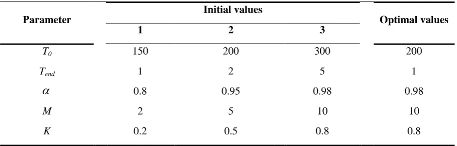
parameters, three levels are considered for each of them and is selected according to the number of the parameters and the levels of design of experiments. Three levels have been determined for each factor (parameter) to design the experiments. In Table 1, the first column represents all of the parameters of SA and the next three columns represent the considered initial values for these parameters. These values have been chosen according to the proposed values in (Glover and Kochenberger 2005). After implementing experiments on the data of Table 1, the average of S/N ratio for 27 levels of Taguchi experiment has been shown in Figure 1. Also, the optimal values of parameters for SA algorithm have been presented in the last column of Table 1.

Figure 1: Average of S/N ratio for parameter adjustment of SA algorithm

Table1: Parameter values of SA

Optimal values Initial values

Parameter

3 2

1

200 300

200 150

T0

1 5

2 1

Tend

0.98 0.98

0.95 0.8



10 10

5 2

M

0.8 0.8

0.5 0.2

K

3.5. Calculating fitness function of generated solutions

To determine the fitness function value of each generated solution by metaheuristic method, firstly the objective function value (which is the total cost of traversed distance by vehicle) is calculated regardless to the solution robustness. Then, the following steps are done:

Step 2. _k number of edges with the highest uncertainty value of demand are selected and their demands are increased into the maximum possible value, according to their demand uncertainty interval.

Step 3. If _kis non-integer, the demand of the last selected edge is increased by(_k  _{ }_k )dˆ. ˆd is defined by multiplying the demand parameter by the deviation level δ (i.e., ˆd d ).

Step 4. With regard to the considered changes in the demand of the edges, if the demand of each edge exceeds the vehicle capacity, a penalty proportional to the violation value is added to the objective function.

4.

Numerical results

In this section, the method of generating different random instances for evaluating the performance of the proposed algorithm is described. Also, the efficiency of algorithm is studied in comparison with CPLEX solver as exact method.

4.1.Generation of random instances

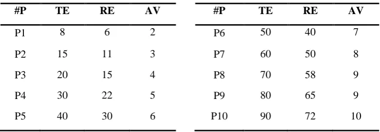
To generate the random instances in different size, n nodes are generated randomly in a two-dimensional coordinate space and node 1 is considered as a depot. Then, a n n matrix is considered to define the available edges in the instances. The value of each cell is one by the probability of 0.7 or zero by the probability of 0.3. One in the matrix, indicates that the edge exists in the instance. Next, 0.7 of the edges are selected randomly as required edges and their demands are generated randomly using uniform distribution U [1,4]. The capacities and number of vehicles are coi data are given in Table 2.

Table 2: Random generated instances

#P TE RE AV #P TE RE AV

P1 8 6 2 P6 50 40 7

P2 15 11 3 P7 60 50 8

P3 20 15 4 P8 70 58 9

P4 30 22 5 P9 80 65 9

P5 40 30 6 P10 90 72 10

In Table 2, TE, RE and AV are the number of total edges, required edges and available vehicles, respectively.

4.2. Efficiency of the proposed algorithm

In this section, the efficiency of the proposed algorithm is studied. The results obtained by solving the robust model by the proposed algorithm and CPLEX solver, are presented in Tables 3 and 4 for two different deviation level of 0.05 and 0.1. CPLEX contains a primal simplex algorithm, a dual simplex algorithm, a network optimizer, an interior point barrier algorithm, a mixed integer algorithm and a quadratic capability. CPLEX, in turn, contains an infeasibility finder. For the problems with the integer variables, CPLEX uses a branch and bound algorithm. A 3600 seconds run time limitation is considered as the stopping criteria and the best obtained solution during this time is reported.

(24)

(SA CPLEX ) / CPLEX

GAP  objective objective objective

Table 3: Comparing results of SA and CPLEX for robust problem with ̂

#P

CPLEX SA

Objective function

Run time (sec)

Objective function

Run time (sec)

GAP

(%)

P1 998 40.4 1016 8.5 1.8

P2 1121 92.0 1154 15.32 2.92

P3 1815 183.5 1865 18.95 2.73

P4 2689 224.1 2743 26.22 2.01

P5 3550 382.6 3644 34.64 2.65

P6 4144 686.2 4211 42.96 1.61

P7 5318 956.6 5428 51.13 2.06

P8 6180 1825.3 6286 60.3 1.72

P9 6756 3014.5 6845 68.17 1.31

P10 7423 3600 7583 77.42 2.16

Ave 3999.4 1100.52 4077 40.36 2.10

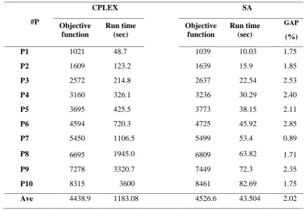
Table 4: Comparing results of SA and CPLEX for robust problem with ̂

#P

CPLEX SA

Objective function

Run time (sec)

Objective function

Run time (sec)

GAP

(%)

P1 1021 48.7 1039 10.03 1.75

P2 1609 123.2 1639 15.9 1.85

P3 2572 214.8 2637 22.54 2.53

P4 3160 326.1 3236 30.29 2.40

P5 3695 425.5 3773 38.15 2.11

P6 4594 720.3 4725 45.92 2.85

P7 5450 1106.5 5499 53.4 0.89

P8 6695 1945.0 6809 63.82 1.71

P9 7278 3320.7 7449 72.3 2.35

P10 8315 3600 8461 82.69 1.75

Results have shown that the proposed algorithm has appropriate efficiency in a reasonable

solution time. Average gaps for the random instances with d 0.05d



 and d 0.1d



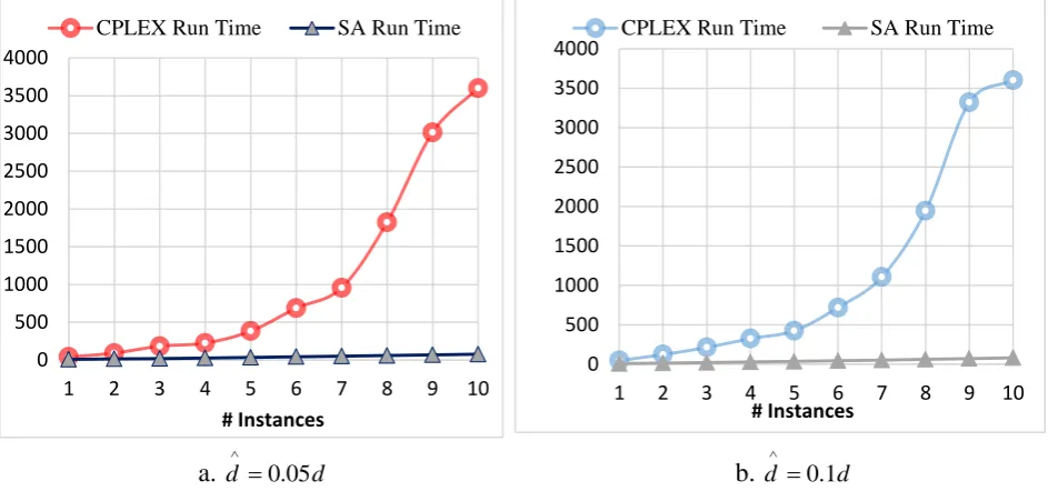
 are 2.1% and 2.02%, respectively. Also, the maximum run time for this algorithm is 82 seconds (P10). The run times of the proposed algorithm and the exact method are shown in Figure 2.

b. d 0.1d

 

a. d 0.05d

 

Figure 2: Comparing run time of SA with CPLEX for solving robust model

As it is clear in Figure 2, deviation level does not affect the run time of the proposed algorithm and the exact method significantly. Also, by increasing the size of the problem, run time of the exact method increases exponentially. But, the run time of the proposed algorithm increases by a linear trend.

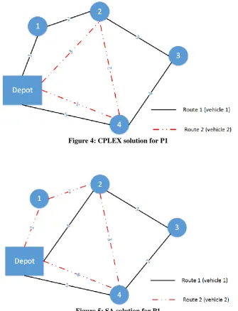
As an example, the solutions obtained by CPLEX and SA for P1 and d 0.05d



 are compared through the figures below. Figure 3 shows a schematic description of P1 including 8 edges with 6 required edges. The solutions obtained by CPLEX and SA have two different routes (Figure 4 and Figure 5), which is the reason why CPLEX reports a little better objective value.

Figure 3: Schematic scheme of P1

0 500 1000 1500 2000 2500 3000 3500 4000

1 2 3 4 5 6 7 8 9 10

# Instances

CPLEX Run Time SA Run Time

0 500 1000 1500 2000 2500 3000 3500 4000

1 2 3 4 5 6 7 8 9 10

# Instances

Figure 4: CPLEX solution for P1

Figure 5: SA solution for P1

Figure 6: Schematic scheme of P2

Table 5: Solutions of P2 for two different deviation level

Depot- 1- 2- 5- 6- 7- 2- 3-6- Depot :Route1 (vehicle 1) Route 2 (vehicle 2): Depot- 7- 6- 5- 4- 3- 2- Depot 0.05

d d

 

Depot- 2- 3- 4- 6- 7- Depot:Route 1 (vehicle 1) Route 2 (vehicle 2): Depot- 1- 2- 5- 2- 7- Depot Depot- 6- Depot:Route 3 (vehicle 3)

0.1

d d

 

According to Table 5, the obtained solution of d 0.1d



 contains three routes with three active

vehicles, while the obtained solution of d 0.05d



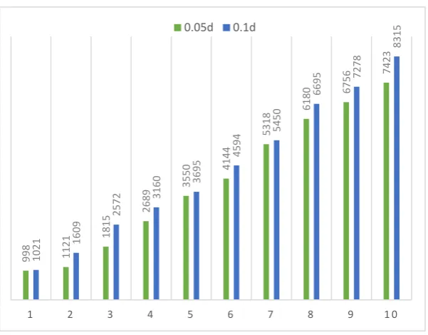
Figure 7: Objective function values with different deviation level

By increasing the deviation level from 0.05 to 0.1, the objective function value of random instances increases by 0.15, in average. In other words, if the manager is interested in protection level of 0.1 than 0.05, he should pay 0.15 more cost, in average. Moreover, the maximum increase of objective function value occurs in problems 2 and 3. In these problems, by increasing the deviation level by 0.05, the objective function value increases about 0.4%.

5.

Conclusion

The optimal routing and allocation of vehicles in CARP is one of the major decisions for organizations such as municipalities in the context of the urban waste collection. The reason is, by optimal allocation and routing of the vehicles they can save vast sum of money. Changes in weekly visit patterns, the occurrence of unexpected incidents and disasters are some reasons which can cause uncertainty in the parameters of CARP. In this paper, a robust mix integer programming model for CARP is developed by taking the demand uncertainty into account. To solve large size problems, a hybrid metaheuristic is used based on the simulated annealing algorithm and a constructive heuristic method. The results showed that the proposed metaheuristic has appropriate efficiency. On the other hand, it was concluded that the problem is sensitive to the deviation level. Therefore, by increasing the deviation level of demand by 0.05, the objective function value increased about 0.15 averagely and it increased even to 0.4% in some problems. For the future studies, more assumptions (like multi trip vehicles, heterogeneous vehicles, etc.) can be added to the problem to make it more applicable in the real world.

References

Beltrami, Edward J., and Lawrence D. Bodin., 1974. "Networks and vehicle routing for municipal waste collection." Networks 4.1: 65-94.

Bertsimas, Dimitris, and Melvyn Sim., 2003."Robust discrete optimization and network flows." Mathematical programming 98.1-3: 49-71.

Bertsimas, Dimitris, and Melvyn Sim., 2004. "The price of robustness." Operations research 52.1: 35-53. Chen, Lu, et al., 2014. Optimizing road network daily maintenance operations with stochastic service and travel times." Transportation Research Part E: Logistics and Transportation Review 64: 88-102.

998 1121

1815

2689

3550

4144

5318

6180

6756

7423

1021

1609

2572

3160

3695

4594

5450

6695

7278

8315

1 2 3 4 5 6 7 8 9 1 0

Chen, Yuning, Jin-Kao Hao, and Fred Glover., 2016."A hybrid metaheuristic approach for the capacitated arc routing problem." European Journal of Operational Research.

Dror, Moshe, and André Langevin, 2000.Transformations and exact node routing solutions by column generation. Springer US,

Fleury, Gérard, Philippe Lacomme, and Christian Prins, 2004. "Evolutionary algorithms for stochastic arc routing problems." Applications of Evolutionary Computing. Springer Berlin Heidelberg. 501-512. Fleury, Gérard, et al., 2005."Stochastic capacitated arc routing problems." Document de travail interne. Article en cours de rédaction

Golden, B., Wong, R., 1981." Capacitated arc routing problems." Network, vol.11, pp.305–315.

Golden, Bruce L., Arjang A. Assad, and Edward A. Wasil., 2001. "Routing vehicles in the real world: applications in the solid waste, beverage, food, dairy, and newspaper industries." The vehicle routing problem. Society for Industrial and Applied Mathematics.

Glover, F.W., Kochenberger, G., 2005. “Handbook of metaheuristics”, Kluwer Academic Publishers, Norwell,

Kirkpatrick, S., & Vecchi, M. P., 1983. Optimization by simmulated annealing. science, 220(4598), 671-680.

Laporte, Gilbert, Roberto Musmanno, and Francesca Vocaturo., 2010. "An adaptive large neighbourhood search heuristic for the capacitated arc-routing problem with stochastic demands." Transportation Science 44.1: 125-135.

Santos, Luís, João Coutinho-Rodrigues, and John R. Current., 2010. "An improved ant colony optimization based algorithm for the capacitated arc routing problem." Transportation Research Part B: Methodological 44.2: 246-266.

Taguchi, Genichi, Subir Chowdhury, and Yuin Wu., 2005. Taguchi's quality engineering handbook. Wiley-Interscience,.

Vincent, F. Yu, and Shih-Wei Lin., 2015. Iterated greedy heuristic for the time-dependent prize-collecting arc routing problem." Computers & Industrial Engineering 90: 54-66.