• No results found

Observation of 2nd Schumann eigenmode on Titan’s surface

N/A
N/A
Protected

Academic year: 2020

Share "Observation of 2nd Schumann eigenmode on Titan’s surface"

Copied!
12
0
0

Loading.... (view fulltext now)

Full text

(1)

www.geosci-instrum-method-data-syst.net/2/237/2013/ doi:10.5194/gi-2-237-2013

© Author(s) 2013. CC Attribution 3.0 License.

Instrumentation

Methods and

Data Systems

Observation of 2nd Schumann eigenmode on Titan’s surface

C. Béghin1, G. Wattieaux1,2, R. Grard3, M. Hamelin4, and J. P. Lebreton1,5

1LPC2E-CNRS-Université d’Orléans, UMR7328, CNRS – 3A, Ave. Recherche Scientifique, 45071 Orléans Cedex 2, France 2LAPLACE-CNRS-Université de Toulouse III, 118 route de Narbonne, 31062 Toulouse Cedex 9, France

3SSD, ESA-ESTEC, European Space Agency, Keplerlaan 1 2200 AG Noordwijk, the Netherland 4LATMOS-IPSL, Université Pierre et Marie Curie, 4, place Jussieu, 75252 Paris Cedex 05, France 5LESIA, Observatoire de Paris- Section de Meudon, 5 place Jules Janssen, 92195 Meudon Cedex, France

Correspondence to: C. Béghin ([email protected])

Received: 28 January 2013 – Published in Geosci. Instrum. Method. Data Syst. Discuss.: 19 April 2013 Revised: 17 September 2013 – Accepted: 29 September 2013 – Published: 22 October 2013

Abstract. This work presents the results obtained from an

updated data analysis of the observations of extremely low frequency (ELF) electromagnetic waves performed with the HASI-PWA (Huygens Atmospheric Structure and Permit-tivity, Wave and Altimetry) instrumentation after Huygens Probe landing on Titan’s surface in January 2005. The most significant signals observed at around 36 Hz throughout the descent in the atmosphere have been extensively analyzed for several years, and subsequently interpreted as the signa-ture of a Schumann resonance, although the latter exhibits atypical peculiarities compared with those known on Earth. The usual depicting methods of space wave data used so far could not allow for retrieving the presence of weak sig-nals when Huygens was at rest for 32 min on Titan’s surface. Whereas the expected signal seems hidden within the instru-mental noise, we show that a careful statistical analysis of the amplitude distribution of the 418 spectral density sam-ples of the 36 Hz line reveals abnormal characteristics com-pared to other frequencies. This behavior is shown to occur under propitious circumstances due to the characteristics of the onboard data conversion processes into digital telemetry counts, namely 8-bit dynamic after logarithm compression of the DFT (Discrete Fourier Transform) of ELF waveforms. Since this phenomenon is observed only at the frequency bin around 36 Hz, we demonstrate that the Schumann resonance, seen in the atmosphere within the same band is still present on the surface, albeit with a much smaller amplitude com-pared to that measured before and a few seconds after the impact, because the electric dipole is thought to have been stabilized ten seconds later almost horizontally until the end of the measurements.

1 Introduction

(2)

2007); and

iii. the first 32 min on the surface, after the Huygens land-ing, up to the pre-programmed switch-off of the HASI-PWA instrument.

The analysis of the three sequences has been performed on the data files (Ref. PWA-Data-Base, 2013) of the DFT ap-plied onboard to the waveform of ELF signals collected by the double-probe boom-antenna (Grard et al., 1995). We then compare the bin at around 36 Hz (hence referred to as bin 36) with the other bins of the spectra. We demonstrate in Sects. 2 and 3 that the peculiarities of the amplitude spectral density (ASD) distribution of bin 36, recorded on the surface, clearly reveal the presence of a coherent natural signal that is other-wise barely visible in the averaged spectral density distribu-tion. These peculiarities are ascribed to the data processing methods applied onboard, namely the logarithmic compres-sion and the discrete quantification of the DFT spectral line amplitudes. Two different numerical simulations (Sect. 4) of the onboard data processing loop are proposed not only to support the SR detection on Titan’s surface, but also to esti-mate its amplitude from signal-to-noise ratio (hence referred to as SNR).

2 Amplitude spectral distribution of PWA-ELF data

The mathematical treatments of the wave field data were de-signed at least ten years before the Huygens landing so as to be performed automatically onboard (Hofe, 2005). The ELF power spectral density (PSD) was computed by apply-ing a DFT after a 16-bit analog-digital conversion of two consecutive waveform samples of 333 ms duration each. The square root of the composite DFT modulus (i.e., the ASD) was logarithmically compressed, and the lower byte (8 bits) was transmitted without the phases to Earth by the telemetry system (hence referred to as TM) via the Cassini orbiter (Le-breton et al., 2005). Therefore, this study is constrained by the limited performances of such usual techniques of wave-data processing of space experiments; nevertheless, we take the best advantage of the proper peculiarities of the PWA-ELF instrument, as briefly described here below. The exper-iment has been operated in two pre-programmed modes, la-beled 131 and 132, dedicated respectively to the high and

are shifted downwards by 1.5 Hz with respect to those of the even bins in mode 131. For instance, bin 36 covers a band-width of 6 Hz, from 31.5 to 37.5 Hz within 3 dB amplitude range (Hofe, 2005). We are then unable to resolve any pecu-liar frequency within that range. Since the aim of this work is rather to identify the presence of a natural signal in bin 36, for the purpose of simplicity we will ignore the 1.5 Hz leftward shift of the frequency scale that concerns the data in mode 132. Hence, a nominal frequency of 36 Hz will be arbitrarily given to bin 36, and similarly to the other bins. Unfortunately, due to the regrettable loss of one of the two TM links (channel A), one half of the original bins were lost, so that only the eight harmonics of bin12 in mode 132 were recovered from the surface data set.

The data are decompressed on the ground according to the transfer function (Jernej and Falkner, 2004), which is valid for both modes,

VADC(ITM)= 4.5 215 10

I

TM−5.1198 32

(volt) (1) whereVADCis the peak amplitude of an equivalent sine-wave signal, with the given frequency injected at the input of the analog digital converter (ADC) and ITM is an integer that represents the lower 8 bits of the log compressed ASD of the average of the two consecutive temporal samples.

A portion of the transfer function is shown in Fig. 1. Since we consider composite signals, the DFT power density of which is assumed to fill up the entire bin frequency band-width, the root mean square (RMS) value remainsVADC/√2 as for sine-waves. The ASDs denoted respectively01and02 in either mode, and the amplitude spectral density of the elec-tric field component received by the antenna in Vm−1Hz−1/2 unit, are given respectively by the following set of equations, 01(131)= VADC

(21f1)1/2

=V√ADC

6

;

02(132)= VADC

(41f2)1/2

=VADC

2

6

;E(f )=01 or 2(f )

leffG(f )

(3)

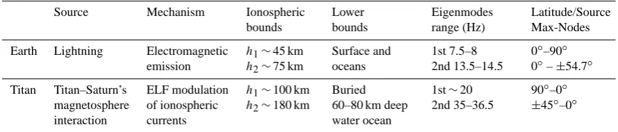
Table 1. Comparison of peculiarities of the Schumann resonances on Earth and Titan (after Béghin et al., 2012).

Source Mechanism Ionospheric bounds

Lower bounds

Eigenmodes range (Hz)

Latitude/Source Max-Nodes

Earth Lightning Electromagnetic emission

h1∼45 km h2∼75 km

Surface and oceans

1st 7.5–8 2nd 13.5–14.5

0◦–90◦ 0◦–±54.7◦ Titan Titan–Saturn’s

magnetosphere interaction

ELF modulation of ionospheric currents

h1∼100 km h2∼180 km

Buried 60–80 km deep water ocean

1st∼20 2nd 35–36.5

90◦–0◦

±45◦–0◦

Fig. 1. Portion of the log-compressed transfer functionVADCversus ITM(Eq. 1).

SR component is assumed to lie (Béghin et al., 2012). Since the precise position of both electric sensors with respect to the local ground is still under investigation, we shall keep in mind for the moment the ratio between the antenna voltages before and after touch down.

It is worth emphasizing here that owing to log compres-sion and the 8-bit quantification, the dynamic range ofVADC is far from linear (Fig. 1). This is the main point that we take advantage of in this work for extracting the weak SR signal from the noise. Even in case of initial normal (Gaussian) dis-tribution, such a non linear process implies that the output decompressed values should exhibit a notably different am-plitude distribution. A bias of the amam-plitude distribution is indeed visible on almost all ELF-PWA spectral data during the descent (Béghin et al., 2009).

In order to prove that this bias is purely experimental and due to the peculiarities of theVADCversusITMtransfer func-tion, we first consider in Fig. 2 the statistical characteristics of the instrument noise measured during the Cruise check-out # 10, labelled above as sequence (i) and performed in the complete absence of natural signal. The bias of a finite series of discrete samples can be defined in different ways (e.g.,

Ghahramani, 2000), but we shall consider here that a distri-bution is biased as long as there is a significant difference between the numbers of samples distributed on both sides of the mean valueµof the series. Note that the mean value be-comes the expectation whenever all samples have the same likelihood, as for instance a noise with a normal amplitude distribution. We shall consider also the quartilesQ1,Q2(or median) andQ3, defined as discrete values of samples split-ting respectively the lowest 25, 50 and 75 % fractions of a series. The bias of the ELF-PWA data is clearly revealed in Fig. 2 (left panel) by the dissymmetry between theQ1 and Q3amplitude bars, that implies a shift between the meanµ and the medianQ2. We say that the bias is positive when-ever the probability in the vicinity ofQ1is larger than that in the vicinity ofQ3. We observe also thatQ2is shifted left-wards with respect toµ. The amplitude vs. time plotted in Fig. 2 (right panel) confirms indeed that most samples lower thanQ2are focused in the vicinity ofQ1. This comes from a substantial excess of moderate and weak amplitude samples which is required to balance the weight of higher values, as a result of the non-linearity of the transfer function (Fig. 1).

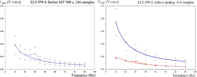
The statistical properties of the data collected during the Cruise checkout #10 will serve as a reference for comparison with situations when weak natural signals are present, such as sequence (ii) during the early phase of the descent and sequence (iii) after landing. These two sequences contain re-spectively 246 and 418 samples of 16 and 8 frequency spec-tra each. The plots in Fig. 3 represent the frequency distribu-tions of the meanVADC RMS amplitudes (µf), plus/minus

one standard deviation (σf)for these two sequences. One

can check that the values ofµf in both modes, 131 and 132,

(4)

Fig. 2. Amplitude distribution (left) and waveform (right) of the first hundredVADCsamples of bin 48 of the Cruise checkout # 10. The bar

levels represent the fractional amount of samples distributed among 6 classes about 6.26 mV RMS wide each, distributed between the min and max values of the series. The solid red line is the theoretical shape of a normal distribution with expectation equal toµ.

Fig. 3. Frequency distribution of two ELF data sequences with the SNR of bin 36 respectively larger (left panel), and smaller than 1 (right

panel). Crosses are mean values and standard deviations. Solid blue lines are LFR fits, excluding bin 36 (see text). Solid red line is the LFR fit of smallest values of the surface sequence excluding bin 36. Dashed lines emphasize the gap between measurements and LFR fits.

In addition to the definitions of the meanµand of the three quartiles, we now recall those of other symbols that will be considered below in order to avoid any confusion with the terminology sometimes used in the literature (e.g., Ghahra-mani, 2000). For large number of samples (N >100) at a given frequency (f), the variance (sf2), and the standard vari-ation (σf), are given by

s2f = 1

N−1

N

X

i=1

(Xi−µN)2 and σf =

q

sf2, (3)

whereXiis the amplitude of an individual sample of indexi,

andµNthe mean amplitude value of the series.Xi represents

either theVADCvoltage amplitude or its RMS value. When the number of frequency samples nf is less than

or equal to 16, such as in the plots of the mean values ver-sus the frequency (Fig. 3), we use the linear flicker regres-sion (LFR) method to fit the most probable analytical func-tion representing the spectral distribufunc-tion of noise in

semi-conductor devices (e.g., Marshall Leach Jr., 1994, and ref-erences therein). Although the classes of different kinds of flicker noises are “as ubiquitous as they are mysterious” after Milotti, (1995), the PSD analytical shape exhibits usually a 1/fβ dependence, withβ growing from 0 to 2 with increas-ing frequency. A transition betweenβ=1.5 and 2 occurs for frequencies such asf >1/2π τ, whereτ is the characteristic time constant of temporal samples. Moreover, note that in our case of ASD data, the shape would be 1/fαwithα=β/2, so

that the LFR function is expressed by

µf =LFR(f )=

A

fα and δ=

1 nf

nf

X

i=1

ABS(xi−µf), (4)

whereA and α are the two coefficients deduced from the mean square regression analysis of a two columns matrix made of nf frequency bins and their associated mean

am-plitudes xi. The quantityδ is the mean absolute deviation

(5)

During sequence (ii), under the large parachute (Fig. 3, left panel), the presence of the signal in bin 36, associated with its side band contribution in bin 30, is well visible above the mean-fit flicker noise with a maximum value of 24 mV RMS. On the contrary, during sequence (iii) on the surface (Fig. 3, right panel), the presence of the signal is barely dis-cerned. The LFR coefficients for the flicker noise are found to beA=0.66 V Hzα and α=0.87, with δ=0.9 mV. Re-porting these coefficients in Eq. (4) leads to a mean fitted valueµf =29.2 mV RMS (i.e., ITM=84) at around 36 Hz (Fig. 3, right panel, blue solid line), whereas the actual mean among the 418 data samples of bin 36 isµ36=30.4 mV (still ITM=84). An increase of 1.2 mV, slightly more than oneδ above the mean LFR instrumental noise, remains however a marginal evidence for the presence of a natural signal in bin 36. We will nevertheless see in the next Sections that this value of 30.4 mV lies just below the jump fromITM=84 to 85, which is a major indicator for the presence of a signal.

We have plotted in Fig. 3 (right panel) the smallest values of each series of 418 samples for all frequency bins of the surface sequence. The LFR fit profile of the smallest values versus the frequency (continuous red plot) is derived from all bins, but the 36 Hz one, in order to avoid biasing the statis-tics with the possible contribution of an additional signal to the noise. One may indeed reasonably assume that the flicker noise contribution at around 36 Hz should not change signif-icantly the global LFR profile derived from other bins. The actual smallest amplitude of bin 36, in terms of telemetry step isITM=72 (i.e., 11.95 mV RMS), whereas the LFR fit in the absence of any signal yieldsITM=69 (9.63 mV). Such increase of 2.32 mV RMS above the LFR profile (Fig. 3, right panel, solid red line), although more significant than that of the mean noise level, does not allow us yet to rule out com-pletely the signature of a purely random event. We now in-vestigate the bias more precisely denoted by the skew of the bin amplitude distribution.

3 Skew versus SNR

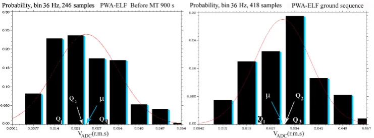
The skew during sequence (ii), before MT 900 s (Fig. 4, left panel), is similar to that observed during the entire descent, and also during the checkout sequence (Fig. 2) used as a ref-erence. Namely, the medianQ2is shifted leftwards with re-spect to the mean value µ, and the amplitude distribution bar in the vicinity of the quartileQ1is higher than that around Q3, which means a positive skew. However, the situation is opposite during sequence (iii), on the surface (Fig. 4, right panel), whereQ2is shifted rightwards and the higher bar is approximately centred onQ3. In addition to singularities of bin 36 discussed in the previous Section, it should be em-phasized that this skew reversal is a remarkable feature that occurs only in the surface data and requires further investi-gation. The conventional definition of skewness for a biased

distribution is given by

G1=

N (N−1)(N−2)

XN

1

X

i−µN

σf

3

. (5)

Applying Eq. 5 to the ELF data throughout the descent yields mean values ofG1of about 0.45, always positive at all fre-quencies including bin 36 (Fig. 9c in Béghin et al., 2009), whereas the same quantity lies in the range 0.16–0.424 dur-ing the surface sequence, with an intermediate value of 0.244 for bin 36. A similar situation holds during the cruise check-out sequence # 10, where the values are distributed between 0.25 and 0.58, withG1=0.36 for bin 36. We therefore con-sider that the conventional definition of skewness does not explain the singularity of bin 36 on Titan’s surface. On the other hand, the shift betweenQ2(a discrete value associated to an integerITM) andµ(a continuous variable) is not a sat-isfying quantitative evaluation of the skew. Indeed, whatever N odd or even, the skew with respect toQ2should depend on the arbitrary choice whether the individual samples of a bin series are considered strictly equal or smaller thanQ2.

We rather prefer an alternative definition for the skew ap-plied to the mean valueµwhich may lie in the vicinity of - but rarely strictly equals- anITM step. Whenever theITM digit increases or decreases by one unit, the quantity |Xi–

µf| exhibits a sudden step in accordance with Eq. (1). As a

consequence, the probability distribution of samples lying in the vicinity ofµf depends on its relative position with

re-spect to the two bracketingITMintegers. We introduce then the skewed standard deviationσf0, an estimator for each

fre-quency bin, defined as σf0=Sfσf with Sf =

N 2Kµf

, (6)

whereSf is denoted normalized skew for any bin series with

the frequencyf, and Kµf is the number of samples of the

series with an amplitude larger than or equal toµf. For a

normal distribution, Kµf ≡N/2 if N is even, andKµf ≡

(N+1)/2 ifN is odd, so thatSf =1 in either case. The

dis-tribution is said to be skewed as long as there is an abnormal excess or deficiency of samples aboveµf. According to the

definition given in the previous Sections, the bias is positive when the skewSf is larger than 1, as observed for most of

(6)

Fig. 4. Amplitude distribution of bin 36 for two sequences for SNR, respectively>1 (left panel), and<1 (right panel).

assume that its own frequency distribution obeys the flicker law. We will then apply here the general linear polynomial regression LPR function

LPR(f )=a+

q

X

1 bq

fq, (7)

whereq is an integer usually smaller than 3 and the coeffi-cientsaandbqare deduced from the least square regression

analysis of a two-column matrix, as done above with the LFR fit.

Though the mean amplitudeµ36of bin 36 during sequence (ii) (before MT 900 s) is well visible above the noise level (Fig. 3, left panel), the plot of the skewed standard deviation σ360 (Fig. 5 left panel) exhibits an even larger jump above the LPR profile. The situation is reversed for the surface data be-causeS36is smaller than 1, thenσ360 < σ36. The best LPR fit applied to the value ofσf0of all bins, but bin 36, which

opti-mizes the mean absolute deviationδ=0.061 mV, is obtained with the following parameters:q=3,a= −1.522 mV,b1= 510.98 mV Hz, b2= −5681.1 mV Hz2, b3=33 450.8 mV Hz3. Introducing these values in Eq. (7) forf =36 Hz, the fit yieldsσ360 =9 mV RMS, whereas the experimental value derived from Eq. (6) is equal to 8.02 mV RMS: about 16δ below the LPR noise measurements in the absence of signal (Fig. 5 right panel, dotted line).

Summarizing the above survey, we retain that the proba-ble presence of a natural signal on Titan’s surface should be identified by three indicators observed only with bin 36 Hz, that are respectively by order of significance: (i) a reversal of skew while the major part of the sample distribution lies in the vicinity of a step of the transfer function, (ii) an ex-cess of smallest values compared to the distribution of other bins, (iii) a weak although noticeable increase of the nominal average amplitude. We therefore propose to reproduce such a behavior and to confirm the fact that the involved mechanism is due to the peculiarities of the onboard data processing and TM transmission. Two different numerical simulations of the entire loop were performed, starting from the ADC input, to the DFT process up to the ground data decommutation.

4 Numerical simulations

The common purpose of the two simulations is to assess the probability of presence of a natural signal in bin 36, and even-tually, to estimate the order of magnitude of SNR. In each simulation we are referring to the same experimental data, with the parameters reported in Table 2. The procedure is basically the same as performed on board Huygens for the mode 132 and we make the following assumptions:

i. in the absence of signal, the instrumental noise spec-trum obeys the LFR function (Eq. 4), with the parame-ters derived in Sect. 2 (A=0.66 V Hzαandα=0.87); ii. the mean spectral characteristics of both signal and noise are assumed to be stationary during the ground sequence;

iii. the amplitude of eachVADCsample (either Volt, mV or RMS, whenever applicable) is the product of its ampli-tude spectral density02by the square root of the bin resolution (Eqs. 1 and 2);

iv. the composite RMS amplitudeA3of both waveforms (noiseA1plus signalA2)at the DFT output reads

A3(VADC)=

A

2

1+A22+2A1A2cosφ12

1/2

, (8) whereϕ12is the differential phase between signal and noise components within the DFT complex plane; v. two successive values for A3 and A3bis are derived

with amplitudes and phases randomly distributed and the resulting average amplitude Â3 is afterward log-compressed and digitized, yielding a value ofITMby inverting Eq. (1);

(7)

Fig. 5. Frequency variation of the normalized skewed standard deviationσf0 for the same sequences as in Figs. 3 and 4.

Table 2. Comparison between the surface data and the retrieved characteristics derived from both numerical simulations.

Bin 36 Mean valueµ(mV) Spread mV (out) σ(mV) Spread mV

VADC RMS Max Min VADC RMS Max Min

Surface data 42.97 30.38 43.1VADC30.45 RMS 42.6VADC30.1 RMS 12.3 8.7 12.6VADC8.9 RMS 11.9VADC8.4 RMS background noise S1 42.86 in 41.3 out 30.3 in 29.2 out 41 3VADC29.2 RMS 41.2VADC29.1 RMS 12.6 in 9.3 out 8.8 12.6VADC8.9 RMS 12.3VADC8.7 RMS bin 36 signal S1 12.8 with SNR=0. 3 9.05 13VADC9.2 RMS 12.7VADC9 RMS 6 with SNR=0.3 4.2 6.6VADC4.7 RMS 5.4VADC3.8 RMS background noise S2 42.4 in 41 out 30 in 29 out 43.8VADC31 RMS 42.6VADC27.5 RMS 12.3 in 11.7 out 8.7 in 13.8VADC9.75 RMS 10.6VADC7.5 RMS

8.3 out composite output S1 expectation 42.85 expectation 30.3 43.05∗V

ADC30.4 RMS 42.6VADC30.1 RMS expectation 12.2 8.6 12.2VADC8.6 RMS 10.5VADC7.4 RMS composite output S2 42.4 30.3 with SNR=0.35 44.1VADC34 RMS 41VADC28 RMS 12.3 8.7 with 13.1VADC9.3 RMS 11.3VADC8 RMS

SNR=0.3

The symbol * means measured skew<1, implyingITM(µ36)<85 (i.e.,µ36<30.45 mV RMS).

vii. the direct transfer function (Eq. 1) is then applied to everyITMsample of each set; and

viii. the global results of two successive series of 100 runs each (simulation S1) or 10 000 runs (simulation S2), are reported below, with the relevant parameters sum-marized in Table 2.

Note that due to the averaging process of two time-independent individual samples (step v), each combined out-putITMvalue is different from that of the original input val-ues. This is the reason why, after completion of the simu-lation processes, the values “out” ofµ andσ of the back-ground noise, in the absence of signal, may differ from the values “in” (Table 2). Such feature accounts for the fact that we are not allowed considering the transfer function Eq. (1) as a biunivocal relation applied through the entire ELF-PWA loop.

4.1 Simulation S1

A first phase of 100 runs has been performed by scanning a wide range of SNR from 0 to 0.6. Three different files of noise amplitudes (A1), 418 samples each, have been com-puted as images of the actual surface noise data bins 12, 24 and 48, after applying the following normalized flicker noise coefficient to the amplitude of each sample

A1=A1f

f

36

α

, (9)

whereA1f is the noise amplitude of thenth sample of the

(8)

Fig. 6. Global summary chart of simulation S1. Highlighted yellow

areas cover the bin 36 experimental ranges of mean amplitudeµ, standard deviationσand normalized skewS, during the ground se-quence. The blue disc (middle panel) demarcates the most probable area for SNR. Green, red and blue crosses correspond to simulation runs based upon surface noise bins 12, 24 and 48, respectively.

The surface sequence contains a significant although lim-ited number (418) of experimental data samples, from which we got the values of µ36=30.38 mV and σ36=8.7 mV (Table 2). The simulations aimed to retrieve values of the same order of magnitude as actually measured, with some margin of uncertainty. In order to estimate this margin we consider that the mean statistical parameters of both sig-nal and noise were staying stationary during the ground se-quence, as usually assumed with terrestrial SRs processing. In such case, the deviations of these parameters should not undergo significant change for a smaller number of sam-ples. We checked indeed that, irrespective of the length of series considered, either the first or the last 200 samples of the surface data, the experimental uncertainties are such that µ=30.3±0.2 mV and σ=8.65±0.25 mV (Table 2), and the skewS36=0.918±0.004. Special attention is paid to the highlighted areas in Fig. 6 just below the step ITM 85

Fig. 7. Distribution of the smallest value of bin 36 derived from

simulation S1; the dark-brown bars correspond to the absence of signal (see text).

where we retrieve satisfactorily the expected values forµ,σ andS36. The self-consistency of these parameters within the spread range of expected values enables us to find out that the most probable range of SNR lies between 24 and 36 % (Fig. 6, middle panel) yielding an expected signal amplitude of 9.05 mV (Table 2) for SNR about 0.3 (Table 2), during the 32 min on Titan’s surface.

(9)

Fig. 8. Distributions of skew numberKµ(left panel) and composite meanµ(right panel) versus SNR (simulation S1). The experimental

values are highlighted by yellow lines.

Fig. 9. Distribution of mean and standard deviation of LFR noise files derived from 10 000 pairs of 418 samples used in simulation S2,

assuming a normal distribution with expected values ofµNandσNequal to 30 and 8.7 mV RMS, respectively.

eigenmode was observed on Titan’s surface from the Huy-gens Probe touch down up to 32 min later.

The second phase of 100 runs allowed also to check an-other aspect of the indicator (i) which occurs whenever the skewSf is smaller than 1 (Fig. 6, lower panel): when the

in-teger numberKµis larger than 209 forN=418 (Eq. 6). We

have plotted in Fig. 8 (left panel) the distribution ofKµas a

function of SNR in the range from 0.22 to 0.36. All points are lying well aboveKµ=209 because these runs were

in-tentionally selected within the experimental data range of µ from 30.1 up to 30.45 mV (Table 2, columns 4 & 5). It appears that the experimental value Kµ=227 (Fig. 8 left

panel), which yieldsSf∼0.92 (Fig. 6, lower panel, yellow

line) might have been obtained for any value of SNR lying in this range. One may however anticipate that for a larger num-ber of runs, the highest probability would rather lie at around Kµ∼222 (i.e.,Sf∼0.94) instead of 0.92, which confirms

that such indicators depend upon the number of data samples. But, the probability forKµ=209 (no signal) is extremely

low (1 % in Fig. 8, left panel).

The last result derived from the second series of 100 runs concerns the indicator (iii) namely, the distribution of the mean composite valueµ versus SNR (Fig. 8, right panel).

The central position (yellow line) of the expected experimen-tal value (µ∼30.3 mV) corresponds to about a 50 % prob-ability for the SNR lying between 0.24 and 0.36, which en-compasses the highlighted range in Fig. 6 and besides em-phasizes the self-consistence between the three indicators identified in Sects. 2 and 3.

4.2 Simulation S2

(10)

Fig. 10. Distribution of mean valueµof the composite bin 36 versus SNR derived from 10 000 runs of simulation S2. The most likely value (SNR∼0.35) lies at the intersection between the green curve and the bright blue line.

i. the noise files with 418 samples each are computed in-dependently from each other by using the statistical pa-rameters (µN andσN)of a random distribution

obey-ing the LFR fit function (Eq.4) with coefficientsAand αderived in Sect. 2;

ii. each composite sample of any series of 418 is derived from Eq. (8) with a constant signal amplitudeA2 cor-responding to a given value of SNR with a random phaseϕ12 where the noise level is the expectation of the global distribution plotted in Fig. 9 (left panel); iii. the only variable quantity for each series of 418

sam-ples is the value of SNR which is scanned from 0 to 0.6 in a large number of runs (10 000); and

iv. for each SNR value, two successive sets of 418 com-posite samples are averaged in pairs, log-compressed and TM converted, as above.

Each file of 418 samples with different background noise amplitudes, introduced in 10 000 different couples, are com-puted according to a normal random distribution obeying the LFR function (Eq. 4) for f =36 Hz, with the expectation µN=30 mV (RMS) andσN=8.7 mV (RMS) at the input

of the loop. Because Eq. (1) is applied successively in re-verse and direct ways, according to the ending remark in Sect. 4, the output values are slightly smaller (i.e.,µN=29

andσN=8.3 mV). Therefore, both sets of values are denoted

“in” and “out” respectively in Table 2. Note that the same ef-fect holds for the simulation S1. From the distributions of µN andσN samples plotted in Fig. 9 one deduces that the

predicted experimental noise (values “out”) on Titan’s sur-face in the absence of natural signal should be characterized by the following parameters

µN=29±1.5 mV RMS and σN=8.3±1 mV RMS. (10)

After performing steps (ii) to (iv), the results are summarized by statistical plots of the distributions of the mean amplitude

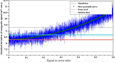
Fig. 11. Distribution of the standard deviationσ of the composite bin 36 versus SNR. The most likely value (SNR∼0.225) lies at the intersection between the green curve and the bright blue line as in Fig. 10. Black lines at 7.3 and 9.3 mV are min and max values, respectively, of noise amplitude in the absence of signal.

of composite signal (µ) and of its standard deviation (σ )in Figs. 10 and 11, respectively. These distributions allow us to confirm that the most likely range of SNR lies between about 0.2 and 0.35, in good agreement with that derived from sim-ulation S1 (Figs. 6 and 8), although both approaches are us-ing different background noise figures. The new information, however, is that the most likely SNR value should be either 0.35 according to the value of the signal composite, or 0.2 according to the standard deviation. We interpret such dis-crepancy as due to much larger uncertainties on the standard deviationσnof background noise than onµn. At the input of

simulation S2, we assumeσn=8.7 mV RMS, with an

over-all dispersion from 7.5 to 9.75 mV (Fig. 9 right panel and Ta-ble 2). As a consequence, the standard deviation of the output composite noise exhibits a total spread of 8–9.3 mV (Fig. 11 and Table 2), whereas the presence of the signal reduces sig-nificantly this spread, thanks to the addition of many values around the composite mean. Therefore, we should rather trust the distribution of the composite mean plotted in Fig. 10, and consider that the most likely value of SNR lies at about 30 %, which reconciles this result with the estimate derived from simulation S1.

5 Discussion and conclusion

(11)

with a most likely value of 0.3 (i.e., a signal of about 9.05 mV RMS within 6 Hz bandwidth at the input of the ADC). Intro-ducing in Eq. (2) the equivalent amplitudeVADC=12.7 mV, the nominal effective length of the antenna (leff=1.6 m) and G(36)=13.5, that is, 22.6 dB volt at 34.5 Hz (Jernej and Falkner, 2004), we obtain an induced electric field strength of about 0.12 mV m−1Hz−1/2. As a useful comparison, this is 10 times less than the last measurements performed during the last phase of the descent and 4 to 6 seconds after touch down (Béghin et al., 2012). However, since the main compo-nent of the conventional SR modes is known to be vertical, the estimate of the actual strength of the incident wave-field vector is most questionable, as it depends on the Huygens motion and tilt of the boom with respect to the local vertical, and whether the sensors are free or in direct electric contact with a lossy dielectric ground (Grard et al., 2006; Béghin et al., 2012).

According to a recent work (Schröber et al., 2012), for about 3 s after touch down, Huygens gondola successively bounced back out of the hole impact, slid and wobbled back and forth five times, after which it commenced a 30–40 cm long slide on a flat surface for about 2 s. During an additional 5 s, the slide motion progressively slowed down until Huy-gens stayed definitely at rest. Because of the ELF-PWA elec-tronic saturation visible on the first two spectra transmitted 2 and 4 s after impact (MT0=8870 s), the first validated data are received at MT=8878.375 s. Since there is a processing-buffering delay of about 2 to 4 s between the acquisition time of the electric field and the MT dating, we may only assume that the first available measurement after impact was per-formed during the first 10 s after touch down. On the other hand, we are essentially concerned with the value of the tilt of HuygensY axis which coincides with the nominal alignment of the PWA boom antenna (Grard et al., 1995). We shall then refer to the measurements performed by the Y-tilt sensor of the Surface Science Package (SSP). After correction of a per-manent minus 8◦offset of this sensor (Leese et al., 2012), we shall consider an average tilt of about 2◦between the nom-inal attitude of our antenna and the local surface during the first 10 s after impact, instead of 10◦initially reported. A tilt of 2◦is consistent with the fact that this value yields the same strength for induced electric field (∼1.2 mV m−1Hz−1/2)as that observed several minutes before impact, as well as a few seconds after touch down (Figs. 2 and 4, in Béghin et al., 2012).

Consequently, our estimate of a signal amplitude ten times smaller during the whole surface sequence after the first 10 s should reasonably lead to a tilt also ten times smaller. How-ever, this is not consistent with the observations of other SSP instruments leading to claim that Huygens was definitely sta-bilized about 10 s after impact (Schröber et al., 2012). For instance, the value measured by the Y-tilt sensor seems to in-dicate still a permanent tilt of 2◦after offset correction. On the other hand, the mutual impedance (MI) device, a compo-nent of the HASI-PWA instrument, designed to measure the

ground conductivity and using partly the same sensors as the ELF dipole antenna (Grard et al., 2006), experienced a regu-lar decay in sensitivity from 10 s after impact before reaching an average stable value (i.e., a behavior compatible with that of the ELF bin 36 data). Such coincidence, still under inves-tigation, could perhaps be caused by some motion of at least one of the boom-antenna without any perceptible influence on the Y-tilt sensor. Alternatively, according to further stud-ies in progress, a slow change in conductivity of the near sur-face, due to the presence of the massive gondola warmer than the dusty surface sediment (Schröber et al., 2012), might ex-plain the simultaneous change of the MI measurements and of the pattern of the local SR wave field.

We have, nevertheless, reached the main objective of the present work which was to identify and quantify the indi-cators which reveal the presence on Titan’s surface of the 2nd SR eigenmode observed during the Huygens descent throughout the atmosphere. We found that the statistical char-acteristics of the bin 36 spectrum data are inconsistent with the normal flicker noise pattern of the other bins, which im-plies that we must reject the option SNR=0 for that bin. Therefore, we estimate that there is more than a 50 % chance that a signal within the frequency range 34.5±3 Hz be per-manently present on the surface, with a SNR of 0.3 (i.e., a mean electric field induced in the dipole antenna of about 0.12 mV m−1Hz−1/2). This value is 10 times weaker than those observed several minutes before Huygens impact and 4 to 6 s after landing. Further work is foreseen, using still pro-gressing investigations on both Titan’s surface global charac-teristics and a presumed slow evolution of the local environ-ment for 32 min after Huygens landing, in order to explain how and why both ELF and MI signals have changed during the first 10 to 15 s after the impact.

Acknowledgements. The authors want to acknowledge the many recognized as well as lowly HASI-PWA team members who made possible the successful achievement of this experiment.

Edited by: L. Vazquez

The publication of this article is financed by CNRS-INSU.

References

(12)

doi:10.1029/2011GL047316, 2011.

Ghahramani, S.: Fundamentals of Probability, 2nd Edn., Prentice Hall: New Jersey, p. 438, 2000.

Grard, R., Svedhem, H., Brown, V., Falkner, P., and Hamelin, M.: An experimental investigation of atmospheric electricity and lightning activity to be performed during the descent of the Huy-gens Probe on Titan, J. Atmos. Terr. Phys., 57, 575–585, 1995. Grard, R., Hamelin, M., López-Moreno, J. J., Schwingenschuh,

K., Jernej, I., Molina-Cuberos, G. J., Simões, F., Trautner, R., Falkner, P., Ferri, F., Fulchignoni, M., Rodrigo, R., Svedhem, H., Béghin, C., Berthelier, J. J., Brown, V. J. G., Chabassière, M., Jeronimo, J. M., Lara, L. M., and Tokano, T.: Properties and Re-lated Physical Characteristics of the Atmosphere and Surface of Titan, Planet. Space Sci., 54, 1124–1136. 2006.

Hamelin, M., Béghin, C., Grard, R., López-Moreno, J. J., Schwin-genschuh, K., Simões, F., Trautner, R., Berthelier, J. J., Brown, V. J. G., Chabassière, M., Falkner, P., Ferri, F., Fulchignoni, M., Jernej, I., Jeronimo, J. M., Molina-Cuberos, G. J., Rodrigo, R., and Tokano, T.: Electron conductivity and density profiles derived from the mutual impedance probe measurements per-formed during the descent of Huygens through the atmosphere of Titan, Planet. Space Sci., 55, 1964–1977, 2007.

Hofe, R.: Signal Analysis of the Electric and Acoustic Field measurements by the Huygens Instrument HASI/PWA. Diploma Thesis, Institute of Broadband Communication, Univ. of Technology, Graz, Austria, p. 163, available at: ftp://lpc2e.cnrs-orleans.fr/users/Christian_BEGHIN/pub/Titan_ papers/HofeDiplomarbeit.pdf (last access; 17 October 2013), 2005.

Huygens surface science package (SSP) : Flight performance re-view and lessons learned, Planet. Space Sci., 70, 28–45, 2012. Marshall Leach Jr., W.: Fundamentals of Low-Noise Electronics,

Proc. IEEE, 82, 1515–1538, 1994.

Milotti, E.: Linear processes that produce 1/for flicker noise, Phys. Rev. E, 51, 3087–3103, 1995.

Nickolaenko, A. P. and Rabinowicz, L. M.: On the possibility of existence of global electromagnetic resonances on the planets of Solar system, Space Res., 20, 82–89, 1982.

PWA-Data-Base: available at: http://atmos.nmsu.edu/PDS/data/ hphasi_0001/ (last access: August 2013), 2013.

Schröber, S., Karkoschka, E., and Lorenz, R. D.: Bouncing on Titan: Motion of the Huygens probe in the seconds after landing, Planet. Space Sci., 73, 327–340, 2012.

Figure

Table 1. Comparison of peculiarities of the Schumann resonances on Earth and Titan (after Béghin et al., 2012).
Fig. 2. Amplitude distribution (left) and waveform (right) of the first hundred VADC samples of bin 48 of the Cruise checkout # 10
Fig. 4. Amplitude distribution of bin 36 for two sequences for SNR, respectively > 1 (left panel), and < 1 (right panel).
Fig. 5. Frequency variation of the normalized skewed standard deviation σ ′f for the same sequences as in Figs
+4

References

Related documents

Biograph mCT’s Adaptive Dose Shield protects the patient from unnecessary pre- and post-spiral radiation, conserving 20% dosage in routine CT exams.With its ultra-low dose

The lessons from the Asian and other financial crises demonstrate that open capital accounts with pegged exchange rate regimes in economies with fragile financial systems and

major determinant of inflation in Ghana. Inflation reduces rapidly till the 3rd and 4th month when the effects begin to die off after the 6th and ih months.. During the

Institute of Electrical and Electronics Engineering (IEEE) 1220, Standard for Application and Management of the Systems. Engineering Process (1994): An

Medicaid Division - Composed of approximately 19 audit professionals, this division performs attestation engagements of financial and statistical reports filed by providers

As the section on purposes set out, assessment data, for the most part based on pupil performance in tests and examinations, are now used in an extraordinary variety of