Optimal Representations of a Traffic Distribution in
Switch Memories
Yaniv Sadeh
Google and Tel-Aviv University, Israel
Ori Rottenstreich
Technion Israel [email protected]
Arye Barkan
Google Haifa, Israel [email protected]
Yossi Kanizo
Tel-Hai College Israel [email protected]
Haim Kaplan
Google and Tel-Aviv University, Israel
Abstract—Traffic splitting is a required functionality in net-works, for example for load balancing over multiple paths or among different servers. The capacity of each server or path implies the distribution by which traffic should be split. A recent approach implements traffic splitting within the ternary content addressable memory (TCAM), which is often available in switches. It is important to reduce the amount of memory allocated for this task since TCAMs are power hungry and are often also required for other tasks such as classification and routing. For splitting a universe of 2W addresses into k pieces of particular sizes, we give a simple algorithm that computes an optimal representation in O(W k)˜ time. Furthermore, we prove that a recently published load balancer, called Niagara, which also runs in O(W k)˜ time is in fact optimal. That is, both our algorithm and Niagara produce the smallest possible TCAM that splits the traffic exactly to the required pieces, where the only previously known algorithm for computing optimal exact representation has running time exponential in k. Finally, we rely on our optimal O(W k)˜ runtime algorithm to investigate through extensive experiments the amount of TCAM memory required to represent traffic splitting in typical scenarios.
I. INTRODUCTION
In many networking applications, the support of traffic split into multiple possible outputs is required. For example, this is required to partition traffic among multiple paths to a destination or when sending traffic to one of multiple servers. The split has to be deterministic such that all packets of the same flow are mapped to a single output, e.g., to avoid packet reordering within a flow. It is increasingly common to rely on the switches in the network to perform the split [1], [2], and traditional schemes use relatively simple hashing techniques for this task. Equal cost multipath routing (ECMP) [3] im-plements a split into k options by associating a hash value with each option and mapping a flow according to the hash value of its flow id. While ECMP distributes traffic uniformly among outputs, in many applications non-uniform distributions are required, e.g., when the outputs differ in their available resources. WCMP (Weighted ECMP) [4] is a generalization of ECMP supporting non-uniform output distributions. The possible output values are written to memory entries with repetitions. Then, a flow is randomly hashed into one of the entries, generating a distribution according to the number of appearances of each possible output.
The implementation of some distributions in WCMP can be costly (in terms of the number of memory entries required).
While for instance implementing a 1:2 ratio can be done within three entries (one for the first output and two for the second), the implementation of a ratio like 1 : 2W −1 is expensive,
requiring2W entries. Memory can grow quickly for particular
distributions for an increasing number of outputs. Moreover, even achieving a distribution similar (under various criteria) to such a distribution might remain expensive.
More recently, a natural approach was taken to implement traffic distributions within the Ternary Content Addressable Memory (TCAM), available in commodity switch architec-tures. For some distributions this allows a much cheaper representation [5], [6], [7]. In particular, a distribution of the form 1 : 2W −1 can be implemented with only two entries. TCAMs are known to be power hungry and thus are of limited size [8], [9]. Accordingly, representations of distributions in TCAMs should minimize the number of required entries.
A related topic is to represent a specific function in a TCAM efficiently (rather than a distribution). Algorithms have been described for finding optimal (prefix-based)1 representation of functions [11]. These algorithms rely on dynamic program-ming in a binary tree structure in which leaves correspond to binary inputs to the mapping. However, the flexibility in the representation of a distribution rules out a simple adoption of algorithms for function representation.
Moreover, finding a representation of a distribution becomes more difficult when the number of possible outputs is large. Wang et. al. [5] consider only a simple encoding without overlap among rules. This restriction unnecessarily results in longer representations than what we can get using overlapping rules and relying on the fact that TCAMs handle rule overlap by ordering the rules. Kang et. al. [6] suggested an algorithm named Niagara, and showed that it is very efficient in prac-tice. Unfortunately they did not prove any guarantees on its performance. Rottenstreich et. al. [7], focused on the case of splitting traffic into two outputs. They described an optimal solution for that case and proved that allocating consecutive interval of addresses to each option is an optimal solution. Moreover, they gave a formula for the cost (number of rules) of an optimal representation of a distribution over two outputs, relating the cost to the number of powers in a signed bit
1Note that finding a non-prefix representation of a function is known to be
representation of the target sizes [12]. The case of multiple outputs was also considered in [7]. They gave an algorithm to compute an optimal solution that requires memory and running time which were exponential in the number of outputs.
Our contributions. We describe an optimal algorithm that finds in polynomial time the minimal size representation of any given distribution (Section III). Moreover, we analyze the existing Niagara algorithm and show that it is also optimal (Section IV). Finally, we provide experiments to evaluate these algorithms (Section V).
Due to space constraints some proofs are omitted.
II. TRAFFICSPLITTINGPROBLEM
A Ternary Content Addressable Memory (TCAM) of width W is a table of entries, orrules, each containing amaskand a target-address(targetfor short). (We assume each target is an integer in[1,2, . . . , k].) Each mask is of lengthW and consists of bits (0 or 1) and wildcards (*). An (IP) addressis said to match a mask if all of the specified bits of the mask agree with the corresponding bits of the address. If several masks fit an address, the first rule applies. An address v is associated with the target of the rule that applies tov. We consider only minimal sets of rules, i.e. sets of rules such that we cannot remove a rule without changing the mapping defined by the set. In the following we refer to a set of TCAM rules simply as a TCAM.
We assume in this paper that wildcards appear only as a consecutive suffix of the mask.2In this setting a mask is in fact a prefix that matches all addresses that start with this prefix. The set of addresses S(p1) and S(p2) that match different prefixes p1 and p2 (assume wlog that p1 is not longer than p2) form a laminar set system. That isS(p1)⊇S(p2)ifp1is a prefix ofp2andS(p1)∩S(p2) =∅otherwise. Furthermore, in casep1is a prefix ofp2then we may assume thatp2appears before p1 since otherwisep2 is redundant. It follows that we may assume that the prefix rules are sorted in a non-increasing order of their lengths. Finally, we assume that our set of rules ends with a match-all prefix (of length 0) that matches all addresses. So there isn’t any address that is not matched by our rules.
A set of prefix rulesT corresponds to a subset of the nodes of the full binary trie.3 In particular, the root corresponds to the match-all prefix, and each prefixpcorresponds to the node whose path to the root corresponds top. The rule which applies to an address v (which is a leaf) corresponds to the closest ancestor which represents a prefix in T. This is the longest prefix of the address v inT.
A TCAM of widthW withk targets partitions the address space of 2W binary strings into k parts. Each address is associated with the target of the rule that applies to it.
2Alternatively, one may assume that wildcards are a prefix of the mask as
in [6]. This may have some practical advantages in certain load balancing settings. In our presentation it is completely symmetric.
3This is a full binary tree of depthWwith2Wleaves, each leafvrepresents
a word ofW bits which corresponds to the path from the root tov, where following an edge to a left child translates to0and following an edge to a right child translates to1.
The problem that we study in the paper is the following. Problem 1. Given k integer weightsx1, . . . , xk that sum up
to 2W, find the shortest TCAM that partitions the addresses intok parts of exactly these sizes.
We observe that a set of prefix rules T that induces a partition into subsets of sizes x1, . . . , xk defines
(non-uniquely) a sequencesof transactionsbetween pairs(i, j)∈
[1, . . . , k]×[1, . . . , k], i 6= j of the form xi ← xi −2`,
xj←xj+ 2` for some integer`, such that after “executing”
sonx1, . . . , xk, all thexi are0except for onexj that equals
2W. Indeed, think of the representation ofT as a binary trie. Consider a prefixpwith targetA such that no descendant of pis inT. Letp0 be the closest ancestor ofpwhich is also in T. Let A0 be the target of p0. By our minimality assumption A0 6=A, so we add to s a transaction moving 2` from A to A0 and removepfromT. Then we iterate this step until only the match-all is left inT.
We refer to a sequence of transactions for x1, . . . , xk that
“sums” all weights into a single weight by moving powers of two as alegal sequence of transactions.
Given a legal sequence of transactions s obtained from a TCAM T as above we can reconstruct T by traversing s in reverse and acting as follows. When we encounter a transaction moving2`fromitoj, we add a prefix rule with targetiwhich
extends a previous prefix rule of targetj. The prefix rule ofi which we add has a subtree of size2` and the prefix of rule
j which we extend has a larger subtree size (it could be an arbitrary one among those).
Note that an arbitrary legal sequences, may not correspond to a set of prefix rules by the transformation above. This may happen when we do not have a rule ofjof the appropriate size to extend, when we get to add a rule for some transaction from itoj. This may happen even ifsis sorted by non-decreasing size of the transactions.
Nevertheless, we define the following related problem. Problem 2. Given an array of k integer weights x1, . . . , xk
where Pk
i=1xi = 2W, compute a shortest legal sequence of
transactions for x1, . . . , xk.
We argued that any TCAM with n rules that induces a partitionx1, . . . , xkalso gives a legal sequence of lengthn−1
for x1, . . . , xk. It follows that if a shortest legal sequence s
for x1, . . . , xk of length m corresponds (using the mapping
defined by the reconstruction process that we described above) to a TCAM of length m+ 1 then this TCAM is a smallest possible among the TCAMs that induce a partition into parts of sizesx1, . . . , xk.
We obtain an algorithm for Problem 1 by giving an al-gorithm for Problem 2 that produces sequences that we can translate to TCAMs.
In order to continue and describe our algorithms and results we introduce the following notations and definitions.
of xchanges by the algorithm the value of this bit may change as well.
(2) [x→`y]: a transaction of size2` from the “sender”xto
the “receiver” y. In accordance with (1) we say that this transaction is at level `.
(3) For our first algorithm we use the following order on the integers. We say that x y or that “x is bit-reversed lexicographic smaller thany” if at the lowest level`where x[`] 6= y[`] we have x[`] = 0 < y[`] = 1 (We assume arbitrary and consistent tie breaking if x =y). We also use the terms lower and higher with respect to this order. We describe two simple algorithms that compute a shortest legal sequence for a given list of weights x1, . . . , xk. Both
can be easily implemented in O˜(W k) (The O˜ hides poly-logarithmic factors). The first algorithm which we propose is new, and is described in Algorithm 1. The second algorithm is the existing Niagara algorithm of [6]. Its pseudo-code (using our terminology) is described in Algorithm 2. Kang et. al. [6] introduced this algorithm4 and demonstrated its empirical effectiveness, but they did not prove bounds on the number of rules that it produces. We prove that Niagara indeed produces a shortest legal sequence given x1, . . . , xk (which can be
mapped to a TCAM).
Consider Algorithm 1 first. It generates a sequencesordered from smaller to larger transactions. From the definition of Algorithm 1, it is clear that no weight participates in more than one transaction of a given size. From this follows that we can mapsto a TCAM since the sum of all transactions of sizes less than2`, per anyx
i, is strictly smaller than2`. Note
that Niagara constructs the sequence in “reverse” order, from the last transaction to the first.
A high level overview of Niagara is as follows. Consider a target partitionP = (x1, . . . , xk)and assume thatxi≤xi+1. We set the target of the match-all prefix to be k. Each step of the algorithm adds a single rule and changes the partition. LetD= (d1, . . . , dk)denote this dynamic partition initialized
to (0, . . . ,0,2W) and that should be equal to the partition P at the end. At the beginning of each step we inspect the vector of differences ∆ = (x1−d1, . . . , xk −dk). Clearly,
if ∆ 6= (0, . . . ,0) then it necessarily has positive as well as negative entries. Let a1 ∈[1, k] be the index of the minimal (negative) difference and a2 ∈ [1, k] be the index of the maximal (positive) difference in ∆. The two differences are xa1 −da1 andxa1 −da2, respectively. We compute a value
λ = 2i such that when moving λ from server a
2 to server a1, theL1norm of∆following this transaction is minimized. Then a transaction moving λ = 2i (with i wildcards) from
servera2 to servera1is added. It follows from Lemma 6 that the sequence produced by Algorithm 2 can be converted to a TCAM.
III. BITMATCHER
In this section we prove the optimality of Algorithm 1 with regard to Problem 2. First of all, it should be noted that since
4As a solution for Problem 1. Problem 2 was not studied.
Algorithm 1: Bit Matcher (in growing order, for finding a shortest sequence)
Input: A partitionP: A List ofk non-negative integer weights that sum to2W.
Output: Shortest sequencesof transactions such that applying it toP yields a list of zeros except for one weight which is2W.
Initializes to be an empty sequence. forlevel`= 0. . . W −1do
LetA be the set of weights whose`th bit is 1(i.e. xi∈A iff bitwisexi&2`6= 0).
SortA in bit-reversed lexicographic order. Pair the weights in Ainto |A|/2 pairs, such that each pair consists of a weight from the first half of Aand a weight from the second half of A.
Make|A|/2 transactions of value2` one per pair,
from the weight of the lower half ofAto the weight of the higher half of A. Apply the transactions on the weights, and concatenate the transactions to s. returns
Algorithm 2: Niagara algorithm [6] overview (following our terminology)
Input: A partitionP: A List ofk non-negative integer weights that sum to2W.
Output: Shortest sequencesof transactions such that applying it toP yields a list of zeros except for one weight which is2W.
Initializes to be an empty sequence, subtract2W from
max(P).
whileP 6= (0, . . . ,0) do
Letx=max(P),y=min(P), and letibe the largest integer minimizing |x−2i|+|y+ 2i|
Apply the transaction[x→iy]and append it to s.
end returns
the sum of all weights is2W, at any iteration, |A| is even. The algorithm ends when all weights are 0 except for one which is 2W (the original sum). Note that we can improve
the complexity of the algorithm by maintaining the order and avoiding re-sorting at every level, but it would be easier to reason about this naive description.
The algorithm described above defines a family of legal sequences all of the same length. We denote this family by S. We refer to a legal sequence of transactions as shortest if it has the minimal number of transactions among legal sequences for given input weights.
Theorem 1. Every sequence in S is a shortest sequence.
how one can transform a shortest sequence into a sequence in S without making it longer, and that all members of S are of the same length.
We assume that the transactions in any sequence are ar-ranged by an increasing order of the level they apply to. I.e. first we have all transactions of size 1, then 2, and so on until 2W−1. Clearly, this reordering can change the intermediate values for some weights after applying a part of the transactions. However, the ordering keeps their final value. We do not restrict the sequences to maintain all the weights positive after each transaction. However, it follows from our arguments that there exists shortest legal sequences that keep all weights positive at all times. 5
Lemma 1. In any shortest sequence, any weight, cannot be both a sender and a receiver at a given level.
Proof. We can replace a pair of transactions [y →` x] and
[x→`z]by the single transaction [y→`z]and get a shorter
equivalent sequence.
Remark 1. By Lemma 1, we may extend the notion of “sender” and “receiver” from a single transaction to a whole level. I.e., in a specific level, x can be regarded either as a sender or as a receiver (or none).
A sequence in S does not contain transactions of the following two types. We refer to such a transaction as a violating transaction.
• zero-transaction:A transaction[y→`x]wherex[`] = 0
or y[`] = 0.
• downward-transaction: A transaction [y →` x] where
x[`] = 1andy[`] = 1butxy.
The next two lemmas show that there exists a shortest legal sequence without zero and downward transactions.
Lemma 2. Letsbe a shortest legal sequence that contains a zero-transaction. Let`be the level of the first zero-transaction
[x→` y] ins. Then, there exists a modified sequence s0 of
the same length as s that has no zero-transactions at levels < `and has one less zero-transaction thansat level`, while not increasing the number of downward-transactions at levels
≤`.
In proving Lemma 2 it can be seen that a zero-to-zero transaction (x[`] = y[`] = 0) is sub-optimal. The other two cases could be optimal, but we can still modify them. Examples:
• case x[`] = 0, y[`] = 1: [x= 2, y = 3, z = 3]could be done by[x→0y][x→0z][y→2z]yielding[0,0,8], but it could also be modified to[y→0z][x→1y][y→2z].
• case x[`] = 1, y[`] = 0: [x= 1, y = 2, z = 1]could be done by [x→0y][z→0y]yielding[0,4,0], but it could also be modified to[x→0z][z→1y].
5To deal with negative values, in referring to the binary representation of
a number (positive or negative)x, we refer to that ofx+ 2φwhereφ≥W.
The valuex+ 2φis always positive for all weights. It can be shown that this
is equivalent to using the 2-complement binary representation of the negative numbers.
Corollary 2. There exists a shortest sequence in which each weight participates in at most one transaction at each level.
Lemma 3. Let s be a shortest legal sequence without zero-transactions. Let ` be the smallest level where s contains a downward-transaction [y →` x] (i.e. where x y). Then,
there exists a modified sequence s0 of the same length as s and the same prefix of transactions at levels< `. Furthermore, s0 has the same transactions at level ` as s, except that we replace[y→`x]by [x→`y].
Proof. Consider the state of right before applying [y →` x]
(after applying all the previous transactions). Since s has no zero-transactions we have that x[`] = y[`] = 1. Given that xy, there is some lowest level L > `, where x[i] =y[i] for `≤i < Landx[L] = 0<1 =y[L]. We split the rest of the proof into cases according to whether the transactions of sfollowing[y→`x]cause carry intox[L]andy[L](additive
carry, in base 2). We note in advance that each modification will exchange the roles ofxandyin some of their transactions, and could generate new downward-violations at levels higher than`.
(1) There is a carry into x[L], and there is a carry intoy[L]: Since all the bits ofxandy are identical at levelsisuch that `≤i < L, we exchange the roles ofxand y in all transactions starting from [y →` x] up to and including
the transactions at levelL−1. This will still cause a carry into levelLin bothxandy, and therefore does not affect the rest of the sequence.
(2) There isnocarry intox[L], and there isnocarry intoy[L]. We apply the argument of the previous case. This time after replacingxandy in the corresponding subsequence we do not get carry intox[L]andy[L].
(3) There is a carry into x[L], and there is no carry into y[L]. As before we can exchange the roles of x and y in the transactions from level ` to level L−1, and now in the modified sequence the carry goes intoy[L]. Let us examine the various cases of the transactions insat level L and show how to complete the new sequence in each case. We divide into six cases according to the transactions involving x and y at level L: the first two consider a transaction betweenxandy, and the next four are all the combinations ofxandy interacting with other weights.
(i) If s contains the transaction [x →L y] then we
remove the transaction [x →L y] (which the swap
of x andy made redundant) and continue with all other transactions ofsat levelLand larger. We get a shorter legal sequence which is a contradiction to the optimality ofs.
(ii) Ifscontains the transaction[y→L x]then the carry
that went into x[L], in fact continues into y[L+ 1] (and maybe even higher) after the swap of xandy. We constructs0 by replacing the transaction[y →L
x] by [y →L+1 x] in s. (If we had a carry into y[L+ 2]ins0, then[y →
(iii) scontains[x→Lz][w→Ly]: We replace these two
by[x→Ly][w→Lz]and apply Case (3i).
(iv) scontains[y→Lz][w→Lx]: We replace these two
by[y→Lx][w→Lz]and apply Case (3ii).
(v) s contains [x →L z][y →L w]: We replace these
transactions by[y→Lz][y→Lw]. A new violation
is created at levelL, but sinceL > `this is ok. (vi) s contains [z →L x][w →L y]: We replace these
transactions by[z→Lx][w→Lx]. A new violation
is created at levelL, but sinceL > `this is ok. (4) There isnocarry intox[L], and there is a carry intoy[L]:
LetK be the lowest level> `such thatx[K] = 0. Given that this case asserts that x[L]receives no carry, K < L. Since K < Ltheny[K] =x[K] = 0. Let us consider the following two cases.
(i) s contains [x →K z]: If y[K] = 0 still, since we
have no zero-transactions it doesn’t participate at this level, so we exchange the roles of x and y in all transactions of level`up to and includingKand get a modified sequence s0 with [x→` y] as required.
This is also true ify[K] = 1and is a sender. It cannot be thaty[K] = 1and is a receiver: assuming it was, WLOG we can assume it receives from x[K], and modify the sequence to exchange the roles ofxandy in levels`up to and includingK−1, while removing completely the transaction [x→K y], contradicting
the optimality ofs.
(ii) s contains [z →K x]: The transaction [z →K x]
starts another carry sequence in x (of length 1 or longer) from levelK up to some level, sayK1. As before given that this case asserts thatx[L] receives no carry, we have that K1 < L. If there is a transaction[z1 →K1 x] we define K2 analogously,
and while there is a transaction [zi →Ki x] we
continue and defineKi+1. We have thatKi< Ki+1 and since there is no carry intox[L]there must be an indexαfor which we have a transaction[x→Kαz]
andKα< L. Then we apply Case (4i) forKα.
Corollary 3. There exists a shortest legal sequence without violating transactions.
Proof. We iteratively apply Lemma 2 and Lemma 3. In each iteration we first clear all zero-transactions using Lemma 2. Then we apply Lemma 3 to remove a downward-transaction from the lowest level that contains such a transaction. This could generate zero- and downward-transactions but only at higher levels. These violations will be cleared in the following iterations.
Up to this point, we showed that there exists a short-est legal sequence without zero- and downward-transactions. Although every sequence in S indeed does not have zero-and downward-transactions, avoiding these transactions is not sufficient for being in S. It remains to show that there exists a shortest legal sequence that at any level the transactions
are such that all senders are from the bottom half and all receivers are from the top half (where these halves are defined by the reverse lexicographic order of the values right before we process this level).
Lemma 4. Letsbe a shortest legal sequence without violating transactions. Assume thatscontains the transactions[z→`x]
and [y →` w] such that z x y w. then we can
get a shortest legal sequence s0 that is identical to s in all transactions at levels≤`except that instead of [z→`x]and
[y→`w]it contains [z→`w]and [x→`y].
By now we are ready to prove Theorem 1.
Proof of Theorem 1. Let s be a shortest legal sequence. By Corollary 3, we may assume it has no zero- and downward-transactions. We apply the following transformation to each level `from the least significant to the most significant.
Consider all the transactions insat level`. If all senders in these transactions are from the bottom half and all receivers are from the top half then we do nothing at this level. Note that this includes the case where we have no transactions and since there are no downward-transactions then it also includes the case of a single transaction.
Consider the case in which there is a transaction such that the sender is not from the bottom half or the receiver is not from the top half. Let [y →` w] be such a transaction in
whichy is from the top half. Since this is not a downward-transaction thenwmust also be from the top half. This implies that there must also be a transaction[z→`x] wherez andx
are at the bottom half. (Similarly, if we assume the existence of [z→`x]wherexis at the bottom half we reach the same
conclusion.) We apply Lemma 4 to the transactions[z→`x]
and[y→`w]. This eliminates two transactions in which both
sender and receiver are from the same half. We repeat this step until there are no such transactions at level `.
As a final note, notice that all the sequences of S are equivalent up-to the way we choose to match the halves at each level, but this choice is a degree of freedom that does not change the length of the sequence.
IV. NIAGARA
In Section II we described the Niagara algorithm for solving Problem 2 of finding a shortest sequence of transactions to sum a given array of k integer weights x1, . . . , xk where
Pk
i=1xi = 2W into one of these weights. In this section we
prove that it computes a shortest sequence. We define for the proof a slightly modified version of Problem 2:
Problem 3. Given an array of k integer weights x1, . . . , xk
such that Pk
i=1xi = 0, compute a shortest sequence of
transactions such that all weights end up as zero.
First we prove that the while-loop in Niagara’s algorithm in fact solves Problem 3. This is stated as Theorem 4.
Theorem 4. Starting with integer weightsx1, . . . , xksuch that
Pk
i=1xi = 0, any sequence generated by the while-loop of
Then, we use it to prove the main result of this section:
Theorem 5. Any sequence generated by Algorithm 2 is a shortest sequence for Problem 2 in whichx1, . . . , xk are such
that Pk
i=1xi= 2W.
Consider now the proof for Theorem 4. We call a sequence of transactions legal if it ends such that all weights are zero. All sequences we talk about in the proof are legal. The Niagara algorithm defines a specific family of legal sequencesS(due to tie-breaking when the mininal/maximal values are not unique). We refer to a legal sequence of transactions as shortest if it has the minimal number of transactions among all legal sequences. We prove that any sequence in S is a shortest sequence. We prove this by showing how to convert any arbitrary shortest sequence into a sequence ofS without increasing its length.
For any given sequences, we reorder the transactions insin a decreasing order of size. This may change the intermediate values of the weights, but it keeps their final values zero. We refer to a sequence ordered this way as anordered-sequence. The structure of the proof is as follows.
(1) First, we prove several lemmas for sequence manipulations that allow us to replace certain subsets of transactions (Lemmas 5 to 6). These substitutions are used for merging small transactions that sum to a power of 2, to create a larger transaction.
(2) Then, we prove that a transaction must happen from a positive weight to a negative weight (Lemma 7), and that it could be between the maximal (positive) and minimal (negative) weights (Lemma 8).
(3) Then, we determine, by case analysis, the size of the transaction that corresponds to the sum of absolute values rule (Lemma 9). There is a specific transaction size corresponding to each case, and Lemmas 10 to 15 show that in each case there is a shortest sequence that starts with a transaction of the appropriate size.
(4) At last, with one additional Lemma (16) we combine everything to prove Theorem 4.
Lemma 5. Let s be a shortest ordered sequence. Consider the situation after performing all transactions of s at levels higher than k, and Let x≥2k be a weight. Then among the
remaining transactions of sthere is a subset in which xis a sender and the transactions’ sizes sum up to exactly 2k.
A similar lemma can be stated for negative weights.
Lemma 6. Let A be some set of transactions [x →mi zi]
such that P
i2
mi = 2`. Then there exists an equivalent set of
transactionsA0of the same size which contains the transaction
[x →` z1]. By equivalent we mean that A and A0 change each weight by the same amount. Similarly, if A is a set of transactions[zi→miy], then there exists an equivalent set of
transactionsA0 which contains the transaction[z1→`y].
Proof. First consider the statement forx. The setA0 consists of the transaction [x→` z1] with the additional transactions
[z1 →mi zi] for i > 1. The statement for y is analogous:
Fig. 1. Sum of absolute values after a transaction as a function ofd(see graph’s title), for the case|y|<|x|.
A0 consists of the transaction [z1 →` y] with the additional
transactions [zi→mi z1]for i >1.
Lemma 7. In any shortest ordered-sequences, any transac-tion[x→`y]satisfies thaty <0< x.
Note that the sequence must be ordered for the lemma to hold. For example, the list [a = 1, b = 3, c = −4] can be zeroed by the shortest sequence[a→0b][b→2c]where both a and b are positive in the first transaction. However, this sequence is not ordered. When we reorder the sequence[b→2 c][a→0 b] we see that in the first transaction c <0 < band in the second transactionb <0< a.
In the following lemma we prove that there exists a shortest sequence which makes a transaction between the maximal and minimal weights.
Lemma 8. Let sbe a shortest ordered sequence. Denote the maximal weightpand minimal weightn. Then there exists a shortest ordered sequences0 whose first transaction is[p→`
n]for some `.
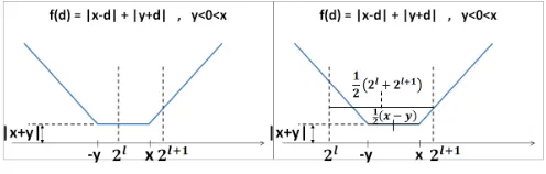
We now proceed to investigate Algorithm 2’s matching rule. Lemma 9. Let y <0< x and let f(d) =|x−d|+|y+d|
for d ∈ R, and for integers k, let g(k) = f(2k). Let m be
the maximum among all minimizers ofg. Fix`such that2`≤
max(x,−y)<2`+1. Then
(1) Ifmin(x,−y)≤2` thenm=`.
(2) Else (i.e. if2`< min(x,−y))thenm=`+ 1ifx−y≥
2`+ 2`+1, otherwisem=`.
Lemma 9 specifies the transaction size that corresponds to the sum of absolute values rule in each of the two cases (1) and (2) that it defines. Here is some further intuition. The function f(d) =|x−d|+|y+d| is piecewise-linear, and its graph is illustrated in Fig. 1 (in the case wherex=−ythe flat segment is of length 0). By definition the value 2`+1 is in the right segment (in which the function has slope 2), but2` could fall
[image:6.612.316.564.50.129.2]The following lemmas correspond to the different cases in Lemma 9 and show that there is a shortest sequence that starts with a transaction of the right size in each of the cases.
Lemma 10. Let s be a shortest ordered sequence, let x ≥
2m be the maximal weight and let y be the minimal weight
before the first transaction. Also assume that |x| ≥ |y|. Then there exists a shortest ordered sequence s0 in which the first transaction is [x→`y], where `≥m.
Note that there are shortest sequences with small transac-tions. For example, the list [8,-2,-2,-2,-2] may be zeroed by applying four transactions of size 2. Lemma 10 proves that it can also be zeroed by applying transactions of sizes 8,4,2,2.
Lemma 11. Letsbe a shortest ordered sequence whose first transaction is [x→`y] wherex≥2m is the maximal weight
andy is the minimal weight. Also assume that|x| ≥ |y|. Then it must be that`≤m+ 1.
Lemma 12. Letsbe a shortest ordered sequence whose first transaction is [x→` y] where x is the maximal weight and
y is the minimal weight. Let 2m ≤ x < 2m+1 and assume
|x| ≥ |y|. If|y| ≤2mthen there exists a sequences0 in which that transaction is[x→my].
Note that Lemma 12 corresponds to Case (1) in Lemma 9.
Lemma 13. Letsbe a shortest ordered sequence whose first transaction is [x→` y] where x is the maximal weight and
y is the minimal weight. Also assume that|x| ≥ |y|. If2m<
−y≤x <2m+1 andx−y= 2m+ 2m+1, then there exists a sequences0 in which`=m+ 1.
Lemma 14. Letsbe a shortest ordered sequence whose first transaction is [x→` y] where x is the maximal weight and
y is the minimal weight. Also assume that|x| ≥ |y|. If2m<
−y≤x <2m+1 andx−y >2m+ 2m+1, then there exists a sequences0 in which`=m+ 1.
An example for Lemma 14 is in order. Consider the list [x, y, z, w, a, b, c, d] = [29,−20,−8,4,−2,−1,−1,−1], where min(x,−y) > 16, x−y >48. One shortest ordered sequence that zeros these weights is:[x→4y][x→3z][w→2 y][x→1 a][x→0 b][x→0 c][x →0 d]. By Lemma 14 there is also a shortest sequence that zeros these weights that starts with a transaction of size 32, for example: [x →5 y][y →3 z][w →2 x][y →2 a][a →0 b][a →0 c][x→0 d]. The latter sequence is derived from the former by first applying Lemma 5 to create a→2 transaction involving x, then increasing the size of the first transaction and lastly exchanging the roles of xandy in some of the following transactions.
Lemma 15. Letsbe a shortest ordered sequence whose first transaction is [x→` y] where x is the maximal weight and
y is the minimal weight. Also assume that|x| ≥ |y|. If2m<
−y≤x <2m+1 andx−y <2m+ 2m+1, then there exists a sequences0 in which`=m.
Note that Lemmas 13-15 cover case (2) of Lemma 9.
We claim that Lemmas 10-15 hold also without the assump-tion that|x| ≥ |y| (the largest positive is greater in absolute value than the smallest negative). The reason for this is that if |x| < |y| we can flip the signs of all weights, and apply the relevant lemma to the flipped set of weights (now the assumption holds sincexandychanged roles,−y is now the largest positive). We get a sequence that zeros the flipped set of weights. If we take this sequence and change the directions of all transactions, we get a sequence that zeros the original weights whose first transaction is as stated by the lemmas. Lemma 16. There exists a shortest sequence whose first transaction is as defined by the Niagara algorithm.
Proof. Lemma 9 specifies what should be the size of the transaction in order to correspond to the minimum sum of absolute value rule that is used by Niagara. Lemma 12 shows that indeed we can start with such a transaction in Case (1) of Lemma 9. Lemmas 13, 14 and 15 show that we can start with such a transaction in Case (2) of Lemma 9.
We are now ready to prove Theorem 4 and Theorem 5.
Proof of Theorem 4. Letsbe a shortest sequence. By Lemma 16 there exists a modified sequences0 whose first transaction adheres to Algorithm 2. Consider the state after the first transaction: this is a new problem of weights that sum up to zero, and the suffix ofs0 must be a shortest sequence of the new problem, otherwise s is not shortest in the first place. Therefore we can repeat and modify s0 so that its second transaction adheres to Algorithm 2. We continue this way, until we reach the end of the sequence, at which point the modified sequence completely agrees with the algorithm.
Proof of Theorem 5. We reduce the original problem to the modified problem as follows: Given a list of integer weights x1, ..., xk that sums up to 2W, we add a new weightxk+1=
−2W. Now we can use the loop of Algorithm 2 to find the
shortest sequence that zeros all the xi’s, denote it by s.
Ac-cording to the algorithm (or by Lemma 8) the first transaction would be [x→W xk+1] wherex=max(x1, ..., xk). This is
the same “dummy transaction” applied in the initialization of Algorithm 2.
Remove the dummy transaction from s, denote this new sequence by s0, and apply s0 to the original weights. For any xi 6= xwhere i ≤k, all of its transactions remain, and
therefore it still ends up equal to zero.xshould have ended up zero with the dummy transaction, thus without it its balance is+2W. We ignorex
k+1 since it was an artificial weight used for the reduction. This means thats0 is a sequence that solves Problem 2. If s0 is not shortest then s is not shortest with respect to Problem 3, which would contradict Theorem 4.
The following Theorem shows how to construct a TCAM from the sequence produced by Algorithm 2.
any level, and it is possible to convert the sequence to a TCAM table.
Proof. Let [x →` y] be some transaction after some prefix
of s has been applied. At this point, xis the largest weight and y is the smallest weight. Let m be the integer such that 2m ≤max(x,−y) <2m+1. By Lemma 9, ` is either m or m+ 1.
If ` =m+ 1: bothx andy flip signs, and from Lemmas 1 and 7 follows that they do not participate in any other transaction of level `.
If`=m: if eitherxoryparticipates in two transactions at level `then by Lemma 1 it either receives or sends a total of 2m+1 and thereby changes its sign and by Lemma 7 cannot participate in any more transactions at that level.
Consider the process of converting a sequence into a trie described in Section II. Since the transactions are ordered by decreasing sizes, when we get to the transaction of level `, all weights in the current distribution are multiples of 2`+1. Therefore any weight that is larger than its target size has a subtree of size at least2`+1 so it can allocate two subtrees of size 2`. It follows that the sequence can indeed be converted
to a TCAM.
V. EXPERIMENTALRESULTS
A. Average number of rules for a partition
In this section we examine the distribution of the smallest number of rules required for partitioning the address space into k parts of random sizes. Since now we have polynomial time algorithms for computing the smallest set of rules, we are able to compute the smallest number of rules for a large number of parts (k) and a large TCAM width (W). This is in contrast with previous work (e.g. [7]) that did not know that Niagara is optimal and only had an algorithm that computes the shortest sequence which is exponential ink.
To compute the distribution of the optimal number of rules, we created100,000random vectors, uniformly distributed over all vectors of length k with a fixed sum of 2W (see [13] for more information on how to generate these vectors using the Dirichlet distribution). Fig. 2 shows the distribution of the optimal number of rules given k∈ {4,8,16}, with a TCAM width of W = 32. This distribution is concentrated around its expectation. For instance, when k = 4and W = 32, the average is∼25.13rules and the standard deviation is∼3.36. Furthermore, it is unlikely to draw a partition that requires less than 19 rules or more than 29 rules. Similarly, whenk= 8and k = 16 the averages are ∼47.41 and∼88.98, respectively. The standard deviations are∼5.50and∼10.43, respectively. B. The length of the address W and the number of partsk
In this section we examine how the smallest number of rules changes with W andk.
Fig. 3 shows the average number of rules, the 10th per-centile, and the 90th perper-centile, as a function of the TCAM width W for a partition ofk= 16 parts. We generated these statistics using10,000 uniformly distributed vectors of length k that sum to 2W for eachW ∈[16,48].
20 40 60 80 100
0 0.1 0.2 0.3
optimal number of rules
probability
k= 4 k= 8 k= 16
Fig. 2. The measured distribution of the optimal number of rules required for an exact partitioning of the address space intok∈ {4,8,16}parts with TCAM widths ofW= 32.
16 20 25 30 35 40 45 48
50 100 150
TCAM widthW
number
of
rules
[image:8.612.323.548.249.334.2]Average 10th percentile 90th percentile
Fig. 3. Statistics of the optimal number of rules required for various values of TCAM widthW given a number of partsk= 16.
20 30 40 50 60
100 200 300
number of partsk
number
of
rules
Average 10th percentile 90th percentile
Fig. 4. Statistics of the optimal number of rules required for various number of partskgiven a TCAM width ofW= 32.
Fig. 4 shows the average number of rules, the 10th per-centile, and the 90th perper-centile, as a function of the number of partskwith a TCAM width ofW = 32bits.
In both cases, the average number of rules required grows linearly withW andk, in Fig. 3 with a slope of∼2.817, and in Fig. 4 with a slope of ∼4.99. Furthermore, the 10th and the 90th percentiles are also close to the average, with a slight gap when the TCAM width or the number of parts increase. This property is extremely important for a network designer who applies traffic splitting using the technique presented in this paper.
C. Approximation using a fixed number of rules
[image:8.612.329.546.380.464.2]bit-matcher algorithm as well as the accuracy of Niagara, when there is a limit on the number of rules.
To measure the accuracy of a given set of rules, we followed [7] and used the single-sidedL∞metric, that is, the maximum difference between the target size of a piece and its actual size, where the maximum is taken over all parts in which the target size is larger than the actual size.
We used the same method described above for creating uniformly distributed fixed sum vectors that sum to 2W. For each such vector, we executed each of the algorithms and tracked the single-sided L∞ distance after the addition of every rule (in our algorithm, we added rules in reversed order, that is from larger subtrees to smaller ones).
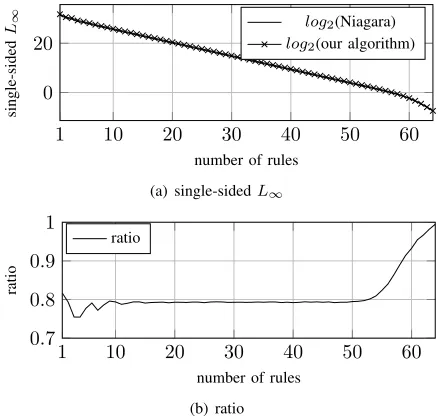
Fig. 5(a) compares the average single-sided L∞ distance of both Niagara and our algorithm over 100,000 random uniformly distributed fixed sum vectors with k = 10 parts and a TCAM width of W = 32bits. Both algorithms behave similarly, but Niagara is slightly better. Fig. 5(b) shows the ratio between the single-sided L∞ distance of the prefix of Niagara’s sequence and the L∞ of the prefix of the sequence produced by our algorithm. This ratio is ∼ 0.79 for most number of rules. When considering single-sided L1 metric, the behavior is similar to Fig. 5 with a ratio of ∼ 0.84. Interestingly, in the corresponding two-sided cases, the ratios stay the same, i.e.∼0.79in the (two-sided)L∞distance, and
∼0.84in the (two-sided)L1distance.
The reason why Niagara performs slightly better with regard to approximations is because our algorithm (Bit Matcher) has degrees of freedom. It is easy to see it through the following example: consider the list[a, b, c] = [1,1,2], and a single rule TCAM. Niagara always assigns the default rule to the largest weight, which iscin this case. In contrast, our algorithm may assign it arbitrarily to any of the weights, depending whether the first transaction is [a→0b] or [b→0a], and whether the next is[c→1a/b]or[a/b→1c]. It is possible to define more carefully how to tie-break when applying the transactions in order to get better approximations.
VI. CONCLUSIONS ANDFUTUREWORK
We introduced a new algorithm for generating a smallest TCAM table for a given partition of an address-space of size 2W. We proved that this algorithm produces the smallest
pos-sible TCAM for this partition. We also proved the optimality of another recently published algorithm that has not been studied theoretically. We used these optimal fast algorithms to experimentally study how the lengths of minimal tables depend on the size of the address-space and the number of servers (number of pieces in the partition). We also studied the error of approximating a distribution by using prefixes of the optimal sequences. This is important in scenarios when the space available is smaller than the entire sequence.
The new algorithm we proposed in this paper can be generalized for bases other than 2, and even generalized further to a “variable base” where all that is required from the set of allowed transaction sizes t0 < t1 < . . . < tn < . . . is
that tj dividesti if j ≤i (this paper covers the case where
1 10 20 30 40 50 60
0 20
number of rules
single-sided
L∞ log2(Niagara)
log2(our algorithm)
(a) single-sidedL∞
1 10 20 30 40 50 60
0.7 0.8 0.9 1
number of rules
ratio
ratio
(b) ratio
Fig. 5. Maximal expense of Niagara and our algorithm given a restricted number of rules withW= 32andk= 10.
ti = 2i). We can prove that these generalized algorithms
produce shortest sequences of transactions. Such sequences may be useful for other applications.
VII. ACKNOWLEDGMENT
The work of Haim Kaplan and Yaniv Sadeh was partially supported by Israel Science Foundation grant no. 1841-14 and the Blavatnik research fund at Tel Aviv University. Ori Rottenstriech is a Taub Fellow (supported by the Taub Family Foundation).
REFERENCES
[1] M. Al-Fares, A. Loukissas, and A. Vahdat, “A scalable, commodity data center network architecture,” inACM SIGCOMM, 2008.
[2] P. Patel, D. Bansal, L. Yuan, A. Murthy, A. G. Greenberg, D. A. Maltz, R. Kern, H. Kumar, M. Zikos, H. Wu, C. Kim, and N. Karri, “Ananta: Cloud scale load balancing,” inACM SIGCOMM, 2013.
[3] C. Hopps, “Analysis of an equal-cost multi-path algorithm,” Nov. 2000, RFC 2992.
[4] J. Zhou, M. Tewari, M. Zhu, A. Kabbani, L. Poutievski, A. Singh, and A. Vahdat, “WCMP: Weighted cost multipathing for improved fairness in data centers,” inEuroSys, 2014.
[5] R. Wang, D. Butnariu, and J. Rexford, “Openflow-based server load balancing gone wild,” inUSENIX Hot-ICE, 2011.
[6] N. Kang, M. Ghobadi, J. Reumann, A. Shraer, and J. Rexford, “Efficient traffic splitting on commodity switches,” inACM CoNEXT, 2015. [7] O. Rottenstreich, Y. Kanizo, H. Kaplan, and J. Rexford, “Accurate traffic
splitting on commodity switches,” inACM SPAA, 2018.
[8] M. Appelman and M. de Boer, “Performance analysis of openflow hardware,”University of Amsterdam, Tech. Rep, pp. 2011–2012, 2012. [9] N. McKeown, T. Anderson, H. Balakrishnan, G. M. Parulkar, L. L.
Peterson, J. Rexford, S. Shenker, and J. S. Turner, “Openflow: Enabling innovation in campus networks,” Computer Communication Review, vol. 38, no. 2, pp. 69–74, 2008.
[10] R. McGeer and P. Yalagandula, “Minimizing rulesets for TCAM imple-mentation,” inIEEE INFOCOM, 2009.
[11] R. Draves, C. King, S. Venkatachary, and B. Zill, “Constructing optimal IP routing tables,” inIEEE Infocom, 1999.
[12] N. J. A. Sloane and S. Plouffe, “The Encyclopedia of Integer Sequences,”
Academic Press, 1995.
[image:9.612.329.551.50.258.2]