https://doi.org/10.5194/gmd-11-3427-2018 © Author(s) 2018. This work is distributed under the Creative Commons Attribution 4.0 License.
The microscale obstacle-resolving meteorological model
MITRAS v2.0: model theory
Mohamed H. Salim1,a, K. Heinke Schlünzen1, David Grawe1, Marita Boettcher1, Andrea M. U. Gierisch1,b, and Björn H. Fock1,c
1Meteorological Institute, CEN, University of Hamburg, Hamburg, Germany anow at: Faculty of Energy Engineering, Aswan University, Aswan, Egypt bnow at: Finnish Meteorological Institute, Marine Research, Helsinki, Finland cnow at: Met Office, Exeter, UK
Correspondence:Mohamed Hefny Salim ([email protected]) Received: 10 October 2017 – Discussion started: 11 December 2017
Revised: 6 July 2018 – Accepted: 10 July 2018 – Published: 24 August 2018
Abstract. This paper describes the developing theory and underlying processes of the microscale obstacle-resolving model MITRAS version 2. MITRAS calculates wind, tem-perature, humidity, and precipitation fields, as well as trans-port within the obstacle layer using Reynolds averaging. It explicitly resolves obstacles, including buildings and over-hanging obstacles, to consider their aerodynamic and ther-modynamic effects. Buildings are represented by imperme-able grid cells at the building positions so that the wind speed vanishes in these grid cells. Wall functions are used to calcu-late appropriate turbulent fluxes. Most exchange processes at the obstacle surfaces are considered in MITRAS, including turbulent and radiative processes, in order to obtain an accu-rate surface temperature. MITRAS is also able to simulate the effect of wind turbines. They are parameterized using the actuator-disk concept to account for the reduction in wind speed. The turbulence generation in the wake of a wind bine is parameterized by adding an additional part to the tur-bulence mechanical production term in the turbulent kinetic energy equation. Effects of trees are considered explicitly, in-cluding the wind speed reduction, turbulence production, and dissipation due to drag forces from plant foliage elements, as well as the radiation absorption and shading. The paper provides not only documentation of the model dynamics and numerical framework but also a solid foundation for future microscale model extensions.
1 Introduction
and to resemble important features of the Earth system such as the Coriolis force effect. Alternatively, high-resolution nu-merical computer models are frequently used to simulate ur-ban areas.
Numerical modeling of wind flow and pollutant dispersion in urban areas is a challenging task due to the geometrical variety of buildings. It inevitably involves impingement and separation regions, a multiple vortex system with building wakes, and jet effects in street canyons (Murakami et al., 1999). Furthermore, the neighbor buildings add their own impacts on the urban meteorology, resulting in interacting flow and dispersion patterns. Due to this complexity, explicit resolving of the buildings is necessary instead of only im-plicitly considering building effects by using surface rough-ness parameterizations. This gave rise to the development of obstacle-resolving microscale meteorological models such as PALM (Maronga et al., 2015), ASMUS (Gross, 2012), ENVI-met (Bruse and Fleer, 1998; Müller et al., 2014), MISKAM (Eichhorn, 1989; Eichhorn and Kniffka, 2010), MUKLIMO (Früh et al., 2011), MITRAS (Schlünzen et al., 2003; Salim et al., 2011), and OpenFOAM (Franke et al., 2012). These models are now widely used for environmental and engineering studies.
The microscale obstacle-resolving transport and stream model MITRAS is part of the M-SYS model system (Truken-muller et al., 2004; Schatzmann et al., 2006). This model sys-tem is designed to investigate pollution transport, chemical reactions, and atmospheric phenomena in the atmospheric boundary layer. The obstacle-resolving MITRAS model cal-culates wind, temperature, humidity fields, cloud, and rain-water, as well as tracer transport within the obstacle layer. The model has been applied for more than 10 years; however, an overall description of the model theory has not been pub-lished in a refereed journal. This is timely because computers now allow for time-dependent long-term integration of the temperature and humidity equations in high resolution. In ad-dition, MITRAS in its version 2 was extended and optimized for more realistic applications in urban areas (Salim et al., 2011; Röber et al., 2013). Specifically, more surface cover classes were added to better describe surface characteristics: fine tuning the code structure for maximum parallelization to make it faster and able to simulate larger domains and pa-rameterizing the additional radiation, turbulence production and dissipation due to wind turbines, and urban vegetation.
Model validations of MITRAS-01 have been performed in comparison to wind tunnel data (Schlünzen et al., 2003; Grawe et al., 2013). MITRAS 2 is evaluated using the VDI guideline for obstacle-resolving microscale models (Grawe et al., 2015). The results will be presented in a separate paper. Equations and the solution method will be described in Sect. 2, including the turbulence parameterization (Sect. 2.2) and numerical treatment (Sect. 2.3). Further sub-grid-scale processes need to be parameterized, even in a very highly resolving atmospheric model like MITRAS. This concerns cloud microphysical processes and radiation. Both are
cal-culated with the same parameterizations as its sister model METRAS (Schlünzen, 2003; Schlünzen et al., 2018b). The boundary conditions, including surface, lateral, and top boundaries, are given in Sect. 3. The treatment of obstacle-induced effects is described in Sect. 4, including wind, shad-ing, and heat transfer effects. MITRAS parameterizes mo-mentum and heat fluxes on obstacle surfaces dependent on the local roughness length (Sect. 4.1, 4.2) and explicitly re-solves obstacles such as buildings, including overhanging ob-stacles (e.g., bridges or overpasses), trees, and wind turbines, to account for its aerodynamics and thermodynamic effects. The handling of wind turbines in the model and their effects is described in Sect. 4.3. Vegetation effects, especially their effect on radiation, are given in Sect. 4.4.
2 Model theory 2.1 Model equations
MITRAS is based on the physical conservation equations, specifically the Navier–Stokes equations, the continuity equation, and the conservation equation for scalar quanti-ties such as potential temperature and humidity. This set of equations is written in flux form, transformed in a terrain-following coordinate system and filtered before it is used in MITRAS.
2.1.1 Coordinate transformation
The equations of MITRAS in flux form are transformed in a three-dimensional nonuniform terrain-following coordinate systemx˙1,x˙2,x˙3so that the lower boundary conforms to the terrain. The vertical coordinate is defined by
˙
x3=zt
z−zs(x, y)
zt−zs(x, y)
. (1)
Here zs(x, y) is the orography height and zt is the
do-main height. The terrain-following coordinates ensure an easy specification of the boundary conditions over orography and eases nesting of MITRAS in METRAS due to the use of the same vertical coordinate transformation. The transforma-tion used allows for grid stretching in all three directransforma-tions to keep a high resolution in the focus area of the domain while allowing some distance between the open boundaries (lateral and top) and the area of interest. In addition, the coordinate system can be rotated against north in any desired angle, al-lowing for additional flexibility. Figure 1 shows an example of a vertical cross section in this terrain-following coordinate system.
2.1.2 Filtering of equations, basic state, and approximations
Figure 1.Vertical cross section to illustrate the MITRAS grid in the terrain-following coordinate system (not to scale). The blue blocks denote buildings. Not all grid cells are shown.
divided into a value ψ, which is the average over a finite time, 1τ, and grid volume, 1x·1y·1z, and its deviation ψ0 (Pielke, 2002). The deviations are assumed to be zero when averaged over1τ. This assumption is reflected in the choice of parameterizations for sub-grid-scale (SGC) turbu-lent fluxes (Sect. 2.2). Performing the filtering operation after the coordinate transformation ensures that all possible fluc-tuations are included with their correct contravariant and co-variant components. The averageψ is further decomposed for temperature, humidity, concentration, pressure, and den-sity into a large-scale partψ0, the so-called basic state, and a microscale deviationψ. The basic state is intentionally cho-e sen to be steady state and fulfill basic concepts of meteo-rology. For example, the base state pressurep0is chosen so that it satisfies the hydrostatic approximation and the vertical gradient is thus balancinggρ0. This ensures a higher order of accuracy when solving the equations, especially for the ver-tical wind. ψo represents a domain average value using the
values at the same height above sea level:
ψo=
1 δxδy
ya+δy Z
ya xa+δx
Z
xa
ψdxdy, (2)
whereyaandxaare the coordinate of a corner of the model andδxδythe domain size in thexandydirection.
To increase the numerical accuracy further, the pressure deviation, pe=p−p0−p0, is decomposed into a quasi-hydrostatic pressurep1(in balance withgeρ) and a more or less dynamically impacted partp2, i.e.,pe=p2+p1. So the pressure can be expressed asp=
e
p=p0+p1+p2+p0. Here p0
e
psop0is neglected.
The Boussinesq approximation is used, and thus density variations in the Navier–Stokes equations are neglected ex-cept for the buoyancy term.p2is determined from an ellip-tic differential equation, which is derived from the anelasellip-tic approximation of the continuity equation, resulting in a de-coupling of pressure and density in the model and hence no sound wave propagation. In addition to the above equations, the ideal gas law and the equation for the potential
temper-ature are solved diagnostically to couple the thermodynamic and aerodynamics of the model.
2.1.3 Solved equations
The solved prognostic equations in MITRAS are as follows. ∂ρ0α∗u
∂t = − ∂ ∂x˙1
ux˙1xρ0α∗u
− ∂
∂x˙2
vx˙y2ρ0α∗u
(3)
− ∂
∂x˙3
˙
u3ρ0α∗
u−α∗x˙x1
∂p 1 ∂x˙1+
∂p2 ∂x˙1
−α∗x˙x3∂p2
∂x˙3+eρα ∗gx˙3
x
∂z
∂x˙3+f ρ0α ∗ v−V
g
−f0d0ρ0α∗w−F1
∂ρ0α∗v ∂t = −
∂ ∂x˙1
ux˙x1ρ0α∗v
− ∂
∂x˙2
vx˙y2ρ0α∗v
(4)
− ∂
∂x˙3
˙
u3ρ0α∗ v
−α∗x˙y2
∂p 1 ∂x˙2+
∂p2 ∂x˙2
−α∗x˙y3∂p2
∂x˙3+eρα ∗gx˙3
y
∂z
∂x˙3−f ρ0α ∗ u−U
g
+f0dρ0α∗w−F2
∂ρ0α∗w ∂t = −
∂ ∂x˙1
ux˙x1ρ0α∗w
− ∂
∂x˙2
vx˙y2ρ0α∗w
(5)
− ∂
∂x˙3
˙
u3ρ 0α∗w
−α∗x˙z3∂p2
∂x˙3
+f0ρ0α∗ ud0−vd−F3
∂ρ0α∗χ ∂t = −
∂ ∂x˙1
ux˙1xρ0α∗χ
− ∂
∂x˙2
vx˙y2ρ0α∗χ
(6)
− ∂
∂x˙3
˙
u3ρ0α∗ χ
+ρ0α∗Qχ−Fχ
Hereu,v, andw are the wind velocity components in the Cartesian coordinates,u˙3 is the contravariant vertical com-ponent of the wind vector,α∗denotes a grid volume, (x˙1,x˙2,
˙
x3), and (x,y,z)are the coordinates of the terrain-following coordinate system and of the Cartesian system, respectively. Ug,Vgdenote the horizontal components of the geostrophic wind,Qχsources and sinks ofχ. The Coriolis parametersf
andf˙are calculated according to the local geographic lati-tudeφand the angular velocity of the Earth’s rotationas f =2sinφandf˙=2cosφ. The variablesd=sinξ and d0=cosξ account for the rotation of the coordinate system by an angleξ against north. The termsF1,F2,F2, andFχ
2.2 Parameterization of turbulent fluxes 2.2.1 Closure for momentum fluxes
Due to the filtering, sub-grid-scale (SGS) fluxes arise. The three SGS turbulent fluxes in the momentum equations (j=
1, 2, 3) are Fj=
∂ ∂x˙1
ρ0α∗u0uj0x˙x1
+ ∂
∂x˙2
ρ0α∗v0uj0x˙y2
(7)
+ ∂
∂x˙3ρ0α ∗
u0u
j0x˙x3+v0uj0x˙y3+w0uj0x˙z3
.
The SGS fluxes can be expressed in terms of the Reynolds stress tensor τij, which is related to the deformation
ten-sor through the turbulent mixing coefficient (Lilly, 1962; Smagorinsky, 1963).
At the lowest model layer, the validity of Monin–Obukhov surface layer similarity theory (Monin and Obukhov, 1954; Foken, 2006) is assumed. The grid-box-averaged values of u∗, θ∗, qv∗ are calculated using stability functions of Dyer (1974) with von Karman constantκ=0.4.
Above the lowermost model layer the SGS turbulent fluxes are derived from a first-order closure (Detering, 1985; Etling, 1987).
τij= −ρ0ui0uj0 (8) =ρ0Kij
∂ui
∂x˙k
∂x˙k
∂xj +∂uj
∂x˙k
∂x˙k
∂xi
−2
3ρ0δijE
Kij is the turbulent exchange coefficient for momentum in
the xj direction. The last term in Eq. (8) represents the
re-duction of the diagonal fluxes due to pressure. Since this term is small compared to the deformation tensor term, it is neglected in MITRAS. Due to the symmetry ofτij, the
ac-tually calculated exchange coefficients are only a horizontal exchange coefficient (Khor) and a vertical exchange coeffi-cient (Kvert).
2.2.2 Closure for fluxes of scalar quantities
The turbulent fluxes for scalar quantities, e.g., potential tem-perature, are expressed as
Fχ=
∂ ∂x˙1
ρ0α∗u0χ0x˙1
x
+ ∂
∂x˙2
ρ0α∗v0χx˙2
y
(9)
+ ∂
∂x˙3ρ0α ∗
u0χ0x˙3
x+v0χx˙y3+w0χx˙z3
.
These fluxes are also parameterized by a first-order closure.
−ρ0ui0χ0=ρ0Kiχ
∂χ
∂x˙k
∂x˙k
∂xj
(10) Kiχ is the corresponding mixing coefficient in thexi
direc-tion, which is related toKij.
The exchange coefficients in MITRAS are either calcu-lated using the Prandtl–Kolmogorov closure (Sect. 2.2.3,
first subsection) or theE–εturbulence closure (Sect. 2.2.3, second subsection). In both turbulence closures the exchange coefficients are calculated as a function of the SGS turbulent kinetic energyE, for which an additional prognostic equation similar to Eq. (6) is solved. For theE–εturbulence closure the dissipationεis additionally calculated from a prognostic equation (López et al., 2005).
2.2.3 Exchange coefficients calculation Prandtl–Kolmogorov closure
The exchange coefficients are calculated as follows. Kvert=c1lE
1/2
f (Ri) (11)
c1 is a free constant determined by matching the theoreti-cal model against experimental values. It has the value 0.55 in MITRAS (López, 2002). The Richardson number Ri-dependent term is defined as
f (Ri)=
1−5Ri forRi>0
(1−16Ri)1/4 forRi≤0, (12) and in accordance with the stability functions used in the sur-face layer. For the SGS turbulent kinetic energy,E, a prog-nostic equation is solved. The dissipation rateis calculated diagnostically as
=cε
E3/2
l . (13)
cεis a constant set to 0.166 (López, 2002). The local mixing
lengthlis related to the stability functionϕmand the distance to the nearest solid surfacezw, which can be the ground
sur-face or a sursur-face of a resolved obstacle. The equation ofl reads
l= κzw
1+κzw
λ
φm. (14)
λis the maximum eddy size (a value of 100 m is used).
E–εturbulence closure
This closure is based on the standard E–ε model and the Kato and Launder (1993) modifications, which eliminate the excessive turbulent kinetic energy produced by the standard E–εmodel in stagnation regions (López et al., 2005). The mechanical production term PM in the E equation can be derived according to the Kato and Launder (1993) modifica-tions as
PM=cµεS. (15)
Sis the dimensionless strain rate.
S=E
ε s 1 2 ∂u i ∂xj +∂uj
∂xi
2
(a) (b)
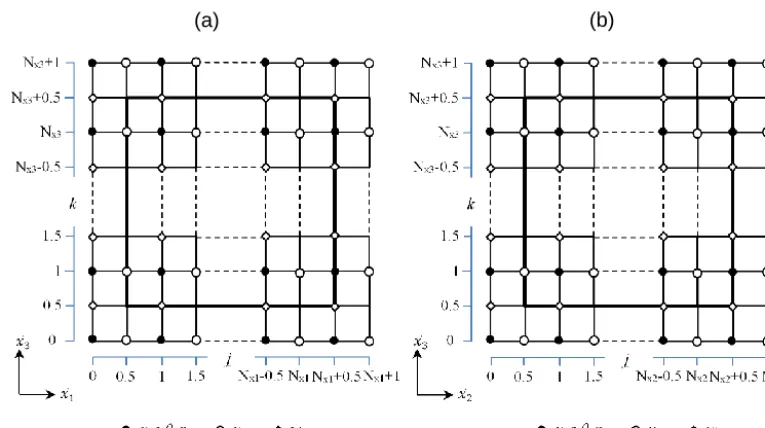
Figure 2.Sketch showing the staggering of the variables of a domain in(a)thex–zdirection and(b)y–zdirection for a model domain with sizeNx1×Nx2×Nx3. The thick line denotes the model domain boundaries. For simplification a uniform grid is shown.
is the rotation rate:
=E
ε s
1 2
∂u
i
∂xj −∂uj
∂xi
2
, (17)
which goes to zero near the stagnation point, soPMis signif-icantly reduced.
It has been shown by Schlünzen et al. (2003) that using Kato and Launder (1993) modifications for both the turbu-lent kinetic energy equation and the dissipation equation in MITRAS leads to overestimation of the momentum fluxes at the stagnation point. To overcome this drawback, they sug-gested limiting the Kato and Launder reformulation to the energy equation only. So, for theεequation, thePMterm is calculated the same way as in the standardE–εmodel.
PM=cµεS2 (18)
The buoyancy term is calculated in the same way as in the Prandtl–Kolmogorov closure. The values for the constants c1,c2,cµ are taken as suggested by López (2005) ascµ=
0.09,c1=1.44,c2=1.92. 2.3 Numerical solution 2.3.1 Discretization
The model equations are solved using finite-volume methods on a staggered Arakawa C grid (Arakawa and Lamb, 1977). On this grid, scalar variables are defined at the cell center, while the velocity components are defined on their respective normal cell faces (Fig. 2). The obstacles faces are set where the corresponding wall normal velocity components are de-fined. Sinceu,v,w, and the scalar variables are defined at
different locations in space, four index arrays are needed to describe the obstacle in the discretized 3-D model domain. The discretization allows for grid stretching in both the ver-tical and horizontal directions to keep focus on the inner part in the domain. The scalar points are always in the center of a grid cell, while the wind components might have different distances to the next-neighbor scalar grid point.
2.3.2 Numerical scheme
The advection and diffusion terms in the momentum equa-tions are solved in MITRAS using the Adam–Bashforth scheme in time and centered differences in space. The vertical diffusion terms are determined using the Crank– Nicholson implicit scheme in order to increase the time step for vertical exchange processes. All other terms in the mo-mentum equations except dynamic pressurep2 are solved forward in time and centered in space.
The dynamic pressurep2is determined iteratively from a Poisson equation to satisfy the anelastic approximation. MI-TRAS allows two user-selected options for the iterative pro-cedures, the iterative IGCG scheme (idealized generalized conjugate gradient; Kapitza and Eppel, 1987) and the precon-ditioned BiCGStab method (biconjugate gradient stabilized; Van der Vorst, 1992).
To avoid numerical artifacts that might appear due to non-linear interactions and result in shortwave energy accumula-tion, artificial diffusivity is added.
Knum=0.5· |U| ·1x·(1−Co)(Roache, 1982), the artificial diffusivity is acceptable in the target area of the domain for two reasons. (a) The isotropic grid and building impacts en-sure advection and diffusion in the horizontal and vertical direction being of comparable size, and (b) advection is of-ten larger than diffusion terms since the SGS turbulence is small within the canopy layer.Uis the local wind speed,1x is the local grid width, andCois the Courant number.
Since Eq. (13) implies that dissipation rate and sub-grid-scale turbulent kinetic energy are directly coupled, the dissi-pation cannot be calculated with very large time steps. Equa-tion (13) is solved by determining an analytic soluEqua-tion (Ap-pendix A) as suggested by Fock (2015). This avoids unphys-ical values ofε, which might even be negative for large time steps1t.
3 Boundary conditions
In MITRAS, several types of boundary conditions can be used in physically consistent combinations to allow for dif-ferent kinds of simulations. At the ground surface (lower boundary) and obstacle faces (Sect. 4) material interfaces are given, while the lateral boundaries and the upper boundary are artificial due to the use of a limited area model.
3.1 Surface boundary 3.1.1 Wind velocity
For the horizontal wind velocity components, a no-slip boundary condition (uj=0,j=1, 2) is used at all vertical
surfaces. With this the vertical wind defined in the staggered grid at the surface also results in zero. Sinceuandvare de-fined at the lowest level atk=0.5 (Fig. 2) on the staggered grid, a Neumann boundary condition is used with a constant gradient using the zero surface values. With this the no-slip condition is achieved at the surface. Additional details for buildings are given in Sect. 4.1.
3.1.2 Dynamic pressure (p2)
The boundary condition for the pressure p2 is formulated by considering the wind velocity boundary condition, the grid staggering, the position of the domain boundaries, and the dynamic pressure equation. Consistent with the no-slip boundary condition, the boundary condition used for p2 at the wall is
∂x˙1
∂x ∂x˙3
∂x ∂p2 ∂x˙1+
∂x˙2
∂y ∂x˙3
∂y ∂p2
∂x˙2 (19)
+
∂x˙3 ∂x
2
+
∂x˙3 ∂y
2
+
∂x˙3 ∂z
2!∂p 2 ∂x˙3 =0.
Due to the terrain-following coordinate system (Eq. 1) the vertical gradient of the dynamic pressurep2needs to be zero perpendicular to the surface.
3.1.3 Temperature
The calculated temperature values of all physical boundaries (ground and obstacles surfaces, i.e., wall and roof) are used at the lower boundary and at the obstacle surfaces. The neces-sary additions for buildings are provided in Sect. 4.2. These temperature values are calculated using the force-restore method for the ground soil heat flux. Following Tiedtke and Geleyn (1975) and Deardorff (1978), the temperature at the surface,Ts, is calculated as
∂Ts ∂t =
2√π κs υshθ
H− √
π υsT−T (−hθ) hθ
!
. (20)
H is the force term of the fluxes of the surface energy bud-get: the net shortwave (RSW,net) and longwave radiation flux (RLW,net), the sensible (QS) and latent heat flux (QL), and the anthropogenic heat emission flux (Qa).T (−hθ)is the
deep soil temperature,hθ represents the depth of the daily
temperature wave in the restore term, andκs is the thermal diffusivity of the surface cover material.
BothRSW,net andRLW,net are calculated using the atmo-spheric radiation scheme of the MITRAS sister model ME-TRAS (Schlünzen et al., 2018b) and the surface characteris-tics, i.e., the albedo value. The influence of vegetation and the shading from the obstacles is taken into account in the calculation of radiation (Sect. 4.4). The fluxesQS andQL are calculated with respect to the thermal stratification using the friction velocityu∗ and the scaling values for heat,θ∗, and water vapor,q∗.
For obstacles, the calculated surface temperature (Sect. 4.2) of the obstacle surfaces is used at the correspond-ing grid cells.
3.1.4 Humidity
The following budget equation, introduced by Dear-dorff (1978), is used to calculate the humidity at the lower boundary (q1s).
class (Sect. 5.2). A prognostic equation is used to calculate αqin the time-dependent model integration.
∂αq
∂t =
QE/ l+P ρwWk
(22) QE is the turbulent humidity flux at the surface (calculated in consistency with QL), l=2.5×10⁶J kg−1 is the latent heat of vaporization of water,P is the precipitation (if any), ρw water density, and Wk is the saturation value for
wa-ter content. This is prescribed for each surface cover class (Sect. 5.2).
3.1.5 Other scalar quantities
At the ground surface and at the obstacle surfaceEandεare calculated as a function of local friction velocity, as follows.
Ez=0= u2∗ c21, εz=0
= u
3 ∗
κz0. (23)
The empirical constantc1 is set to the same value as in Eq. (11). This helps together with Eq. (12) to obtain continu-ous fluxes at the top of the lowest model cell, which employs the surface layer scheme (Lopez, 2002; Fock, 2015). 3.2 Lateral boundary
3.2.1 Wind velocity
Dirichlet boundary conditions are used in two different for-mulations. They can be used in MITRAS in arbitrary com-binations to describe the lateral boundaries of the domain: open boundary (radiative) and fixed boundaries. The appro-priate combination of boundary value calculations depends on the application. For instance, a realistic application with comparison to field data in mind needs open boundaries. In these the boundary normal wind components are calculated as far as possible from the prognostic equations. The bound-ary normal advection is treated with the use of the Orlanski condition at inflow boundaries and by the upstream scheme at outflow boundaries. For the boundary parallel velocity com-ponents a zero-flux condition is assumed (Schlünzen, 1990). When comparison with wind tunnel measurements (e.g., Grawe et al., 2013b) is performed, fixed boundaries are ad-vantageous. In these the wind profiles are to be imposed at the inlet boundary and kept fixed at the initial values, while at the outflow the wind velocity is treated as an open bound-ary.
3.2.2 Other variables
The normal gradients of pressurep2, temperature, humidity, and concentrations are set to zero at the lateral boundaries.
3.3 Top boundary 3.3.1 Wind velocity
For the vertical wind, which is defined at the model top, the Dirichlet condition is used, prescribing it to initial values (mostly vertical wind zero). For all other variables a Neu-mann boundary condition is employed for which the gradi-ents normal to the boundary are zero. In order to avoid re-flections of vertically propagating waves at the upper model boundary, Rayleigh damping layers (absorbing layers) are used in MITRAS. The Rayleigh damping terms, which are added to the flow equations (Eqs. 3–6), are written here. R1= −ρ0α∗ u−UgνR (24) R2= −ρ0α∗ v−Vg
νR (25)
R3= −ρ0α∗wνR (26)
UgandVgare the geostrophic wind velocity components and vRis the relaxation coefficient, defined as
vR=
0 fork < kD
δ(kt−k) fork≥k
D.
(27) k denotes the vertical grid point index,kt the index of the
highest grid point at the upper boundary, andkDthe index of
the first absorbing layer. The coefficientδ is set to 0.2 and, based on our experience, five damping layers are sufficient. 3.3.2 Other variables
The normal pressure gradient, temperature gradient, turbu-lent momentum fluxes, and their gradients are all set to zero at the upper boundary. This assumption results in zero verti-cal heat and moisture fluxes as well as zero momentum fluxes at the upper model boundary.
4 Treatment of obstacles 4.1 Buildings
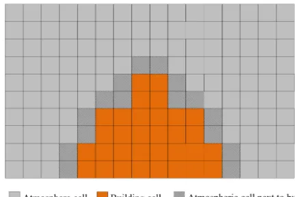
Figure 3.Masking concept in MITRAS.
building surfaces, and grid cells within buildings, as shown in Fig. 3. This separation facilitates the model coding and economizes the computational requirements.
A building mask containing these data is prepared by the preprocessor GRIMASK (Sect. 5.3). In the model, e.g., the wind velocity components vanish at the building boundaries by multiplying the fluxes with the face markers (imperme-able walls). Additional wall functions are included to address friction effects properly.
Building surfaces influence the ambient air temperature. Their effect is taken into account by simulating the sensible heat flux. In grid cells that are adjacent to building surfaces, the termQθ is added to the turbulent fluxes of heat (Eq. 9).
Qθ= −ub∗θb∗ (28)
represents the temperature flux, which is calculated from the friction velocity at buildings,ub∗, and the scaling value for
potential temperature,θb∗.ub∗is calculated following the
ap-proach of Lopez (2002) as ub∗=κ
|vb| lndb zb,0
, (29)
assuming a logarithmic wind profile with neutral stratifica-tion over the building surface.|vb|is the wind speed parallel to the building surface at the first scalar grid cell next to the building surface, i.e., in the distancedb.zb,0is the roughness length of the building surface. The scaling value for potential temperature at buildings is calculated as
θb∗=κ
θd,b−θb
ln db zb,0,θ
(30)
from the difference of the building surface temperature,θb, and the temperature at the first grid cell next to the build-ing,θd,b. The roughness length for temperature at the build-ing (zb,0,θ)depends on the Reynolds number,Re. Following
Brutsaert (1975), the roughness length ratio is calculated as zb,0
zb,0,θ
=expκ7.3Re1/4
√
Pr−5, (31)
with the Prandtl number (Pr) set to 0.71.
This concept allows for a consideration of not only surface-mounted buildings but also overhanging obstacles such as bridges and overpasses or pathways to courtyards. They can all be considered in complex urban geometries. 4.2 Building surface temperature
In order to obtain an accurate surface temperature of the buildings (obstacles), most exchange processes at the build-ing surfaces are considered in MITRAS, includbuild-ing turbulent and radiative processes (Gierisch, 2011). Thus, the physical properties of the façade and wall materials are to be intro-duced as model inputs. These properties include reflectivity, emissivity, heat transfer coefficient, and specific heat capac-ity.
The surface temperature of a building surface,Tb, is calcu-lated from the energy budget of the infinitely thin outermost slab of the building façade. The slab is heated or cooled from outside by a heat sourceHand supported from inside by the rest of the façade that is connected to the building interior. The latter is assumed to be maintained at a temperatureTin.
The rate of temperature change of the slab is governed by the imbalance between the forcing termH and a restoring term. The prognostic equation for the surface temperature reads
cwallD ∂Tb
∂t =H− λ
D Tb−Tin
. (32)
Here the forcing termH is calculated from
H=RSW,abs+RLW,abs−εσ Tb4+QS+QL. (33) RSW,abs andRLW,abs are the absorbed incoming shortwave and longwave radiation,QSandQLare the sensible and la-tent heat fluxes at the surface, which are calculated from the local friction velocity and the local scaling values for temper-ature and humidity (Gierisch, 2011),λis the thermal conduc-tivity,Dis the wall thickness, andcwallis the wall volumetric heat capacity.
The surface energy balance for the inside wall surface can be written as
QC−hi Tin−Troom
=0. (34)
hiis the heat transfer coefficient for the internal wall,QCthe heat conduction flux through the wall calculated asQC=
λ
D Tb−Tin
, andTroomis the room temperature. From Eq. (34), the relation betweenTinandTbis
Tin= hi
hi+ λ D
Troom+ λ D
hi+ λ D
Tb. (35)
Substituting forHandTinin Eq. (32) yields ∂Tb
∂t = 1 cwallD
The right-hand side of Eq. (36) is a function ofTb. Thus ∂Tb
∂t =F Tb
. (37)
Solving Eq.(37) numerically, FTb
t+1t
=FTb
t
+ ∂F
∂Tb T
b
t
Tb
t+1t −Tb
t
, (38)
and solving forTtb+1t gives the time-dependent equation for the surface temperature:
Tbt+1t=Tbt+
FTbt
1
1t − ∂F ∂Tb T
b
t
. (39)
4.3 Wind turbines
Wind turbines are represented in MITRAS by impermeable grid cells at the position of the tower and the nacelle, similar to other buildings (i.e., vanishing wind speed and zero tur-bulent kinetic energy are assumed at grid points within the tower and nacelle). The orientation of the nacelle changes in relation to the wind direction during the model simu-lation. The wind turbine rotor is parameterized by using the actuator-disk concept (Molly, 1978; Mikkelsen, 2003; El Kasmi and Masson, 2008). In this concept the rotor is re-placed by an imaginary permeable disk subjected to a distri-bution of forces that acts upon the incoming flow at a rate defined by the period-averaged kinetic energy that the rotor extracts from the atmosphere.
According to the actuator-disk model, the reduction of the wind speed is caused by the rotor thrust,T, which is formu-lated as
T =1
2cTρAV 2
1. (40)
V1 is the speed of the approaching flow at wind turbine level, Ais the rotor area,ρ is the air density, andcT is the nondimensional thrust coefficient for the corresponding wind speed. The wind speed deficit is limited to those cells located at the actual rotor position. The speed of the approaching flow is calculated with respect to the orientation of the ro-tor, which depends on wind direction and changes direction during the simulation. The thrust coefficient depends on wind speed and therefore the wind turbine automatically switches on and off in MITRAS at the cut-in and cutoff wind speed, respectively.
This wind turbine rotor blades create wake vortices of the wind turbines, which are associated with increased turbu-lence intensity. The turbuturbu-lence generation in the wake is pa-rameterized in MITRAS by adding an additional term,Qwt, to the turbulence mechanical production,PM, in the turbulent kinetic energy equation to account for the turbulence gener-ation at the rotor position. This term is formulated as Qwt=1
2cwtu 2
wt. (41)
uwt is a scale velocity used to characterize the turbulence. The factorcwt(s−1) includes the wind turbine characteristics that govern the amount of produced turbulence, namely the rotor size, the number of blades, and the rotational speed.
In MITRAS, the tangential velocityvθ, which is frequently
used to model the vortex developing behind an aircraft, is used as the scale velocity. The Rankine vortex model (Gerz et al., 2001) is applied here to calculatevθ.
vθ=
0O
2π rc (42)
rc is the vortex core radius and0O is the rotor circulation,
which is related to the rotor rotational speed, lift coefficient, and aspect ratio. More details about modeling the wind tur-bines in MITRAS are given in Linde (2011).
4.4 Vegetation
There are two modes of vegetation treatment in MITRAS: the implicit mode and the explicit mode. In the implicit mode, the effect of the vegetation (grass, bushes, trees, etc.) is im-plicitly considered in the surface parameterization using the roughness length. This is done by allocating the vegetation surface cover class for the corresponding surface grid cells and using the corresponding input parameters (e.g., rough-ness length, soil water, content, etc.; Sect. 5.2).
In explicit mode, vegetation effects are explicitly resolved. These effects include wind speed reduction (Schlüter, 2006), turbulence dissipation due to drag forces from plant foliage– atmosphere interaction (Salim et al., 2015), and radiation ab-sorption and shading.
The wind speed reduction is parameterized by introducing a local three-dimensional sink term,Sui, withi=1, 2, and 3
for theu,v, andwcomponent.Suiis added to the momentum
equations (Eqs. 3–5). Following Liu (1996), the sink term is calculated as
Sui= −cdLAD
˙
x3·U·ui. (43)
Herecdis a drag coefficient,Uis the mean wind speed at heightx˙3, and LAD(x˙3)is the equivalent leaf area density of the plant at heightx˙3. The value ofcd=0.2 determined by Katul (1998) is chosen here.
Sui represents a source of turbulence due to the extraction
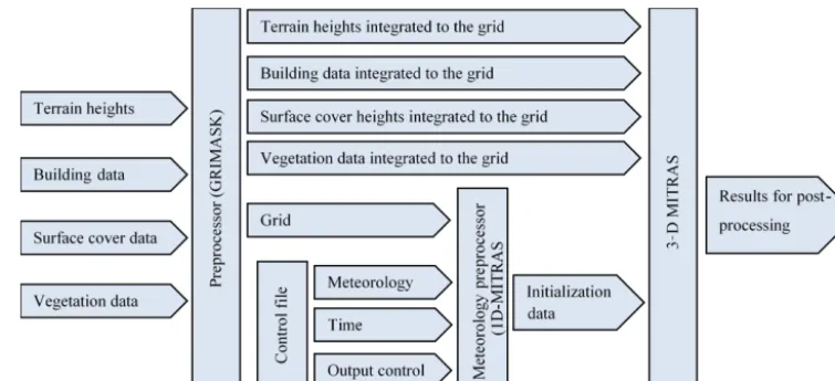
Figure 4.Principal elements of the MITRAS model inputs.
al. (1996) these terms read as follows. Qveg,E=cdLADx˙3
·U3−4cdLADx˙3
· |U| ·E (44) Qveg,ε=1.5cdLAD
˙
x3·U3−6cdLAD
˙
x3· |U| ·ε (45) The reduction of the shortwave radiation flux is considered by including local reduction coefficients (ranging from 1 to 0) according to the vegetation characteristics. The reduction coefficients are described in terms of the vertical leaf area index, LAI, of the plant (see Sect. 5.4).
σSW
˙
x3=expF·LAIx˙3 (46)
5 Model input
Several model inputs are required to run MITRAS to accu-rately simulate a domain for, e.g., an urban area (Fig. 4). These include, for instance, the orography heights of the do-main, the surface cover types, the building data (dimensions, shape, and position), and the vegetation data for such a do-main. Integrating these inputs to the computational domain of MITRAS is done in a separate preprocessor called GRI-MASK (Salim, 2014). A complete description of this pre-processor is outside the scope of this paper, but the required input data and how they are in general achieved is outlined here (Sect. 5.1–5.4). Moreover, the representative meteoro-logical conditions for the domain are required as inputs to run MITRAS; they are provided in consistency with the model physics and numeric using a preprocessor.
5.1 Orography height
Urban domains might include elevated terrain. To better de-scribe the domain terrain, the orographic effects of the do-main are considered in MITRAS by virtue of the terrain-following coordinate system (Sect. 2.1). Both the aerody-namic and the radiative (shading) effects of the slopes are
considered in MITRAS. For realistic applications, the orog-raphy data (terrain height above sea level) of the domain are introduced to GRIMASK in the standard ASCII grid for-mat of a geographic inforfor-mation system (GIS). Usually these data are in much finer resolution (less than 0.25 m) compared to the computational domain horizontal resolution (∼1 m). GRIMASK then aggregates these data to the surface grid cells to calculate the average orography height for each sur-face grid cell. This is done by splitting each grid cell inton grids and calculating the orography height of each sub-grid. The eventual orography height,zs, of a grid cell (i, j )is calculated from
zs(i, j )= 1 n
n
X
1
zsub(x, y) . (47)
zsub(x, y)is the orography height of a sub-grid.
For idealized studies and test cases, GRIMASK can gen-erate artificial orography heights according to the objective of the test case, e.g., a bell mouth hill or a Gaussian hill. 5.2 Surface cover
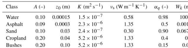
Table 1.The physical parameters for some surface cover classes as used in MITRAS: albedo (A), roughness length (z0), thermal diffusivity
(K), thermal conductivity (νs), soil water availability (αq), and saturation value for water content (Wk).
Class A(–) z0(m) K(m2s−1) νs(W m−1K−1) αq(–) Wk(m)
Water 0.10 0.00015 1.5×10⁻⁷ 0.58 0.98 100.0 Asphalt 0.09 0.0003 2.3×10⁻⁶ 1.35 0.5 0.0015 Sand 0.10 0.03 2.4×10⁻⁷ 0.30 0.90 0.0677 Cropland 0.20 0.04 5.2×10⁻⁶ 1.33 0.4 0.6 Bushes 0.20 0.10 5.2×10⁻⁶ 1.33 0.15 0.06
approach used to calculate the orography heights. Each grid cell at the surface is divided into sub-grids and the surface cover class of each sub-grid is defined. The data structure of the surface cover consists of two datasets: (a) the por-tion of each surface cover class in each grid cell and (b) a list of surface cover classes existing in the domain. Several classes are also prepared in the surface cover class database for the different vegetation types (coniferous trees, decidu-ous trees, bushes, etc.). A database of several surface cover classes with attributed physical parameters is available in the 1-D MITRAS model. The physical parameters given per sur-face cover class include albedo (A), roughness length (z0), thermal diffusivity (K), thermal conductivity (νs), soil water availability (αq), and saturation value for water content (Wk).
The physical parameters are given in Table 1 for selected sur-face cover classes.
For buildings the explicit treatment is normally chosen. If the implicit consideration of obstacles is chosen, i.e., they are not explicitly resolved in the model grid, a much larger roughness length would be required, which conflicts with a high vertical grid resolution. This is similarly true for trees. The roughness length for water is modified during the model calculations with dependence on wind speed (Fischereit et al., 2016). The roughness length of scalar quantities over wa-ter,z0a, is calculated dependent on the roughness length for momentum,z0(Brutsaert, 1975, 2013),
z0(x, y) z0a(x, y)
=expκ
7.3Re1/4pCa−5, (48)
for temperature and humidity by substituting Ca with the Prandtl numberPr=0.76 and the Schmidt numberSc=0.6, respectively.
To distinguish surface cover classes, water, buildings, and sea ice, identifiers are incorporated for each surface cover class. These act as the Kronecker delta function to mark the particular class.
5.3 Building data
In order to generate the building mask used to provide the building data to the model, detailed information about the buildings in the domain is required. For instance, the building dimensions, shape, and location are needed for each building
located in the domain to calculate the 3-D array volume and the building wall-based markers discussed in Sect. 4.1. This process is done in the preprocessor, GRIMASK, which allo-cates the buildings to the computational grid.
Since in the current version of MITRAS the 3-D field vol-ume can be either 0 (building cell) or 1 (atmosphere cell), buildings are approximated to fit into the grid. For grid cells that are partially filled with buildings, the determination of whether these cells are building or atmosphere cells depends on how much volume of the cell is filled with building. A grid cell is considered a building cell if at least 50 % of its volume contains building. Otherwise it is counted as an atmosphere cell. This approximation is computationally efficient to con-sider the effect of buildings since the model equations only need to be multiplied by the 3-D field volume.
For realistic applications, complex urban building geom-etry can be provided to GRIMASK in either the raster digi-tal elevation model (DEM) format, which is commonly used due to the advances in remote sensing technologies, or in the ASCII 3-D computer-aided design (CAD) format. GRI-MASK integrates the high-resolution DEM data, which is a grid of squares representing the elevation of each small grid, to the computational grid and calculates how much volume of the building is contained in each grid cell. When the build-ing data are provided in the ASCII CAD format, GRIMASK uses an approach similar tozbuffering to integrate the build-ing surfaces (usually triangles) to the computational grid and calculates the array volume and the face markers.
5.4 Vegetation
follow-ing relation is used to relate LAD and LAI.
LAIx˙3+1z= z+1z
Z
z
LADx˙3dz (49)
In the analytical approach, GRIMASK uses the following empirical relation proposed by Lalic and Mihailovic (2004) to describe LAD profile from plant parameters.
LADx˙3= (50)
LADm
h−zm h− ˙x3
n exp
n
1−h−zm
h− ˙x3
LADmis the maximum LAD,his the plant height abovezs, zmis the corresponding height abovezs, and
n=
( 6 0≤ ˙x3< z m 1
2 zm≤ ˙x
3< h. (51)
The plant parameters used in these equations can be ob-tained from the forest phenology calendar.
5.5 Meteorology
A large-scale surface-friction-free meteorological situation is required as input to MITRAS to calculate the microcli-mate of a certain domain. This input is prepared by a one-dimensional model without explicit consideration of build-ings but with inclusion of all relevant turbulence processes (including surface friction and Coriolis force) to provide the required meteorology data needed for the initialization of all the variables in the three-dimensional model. Among the in-puts for the one-dimensional model are the large-scale speed wind components, which are taken to be the geostrophic wind and should not include any frictional effects or wind rotation with height that will both be imposed by the 1-D model, the large-scale potential temperature gradient or temperature profile, the large-scale relative humidity profile, the deep soil temperature, and the number of days without precipitation (dry days) prior to the simulation. The one-dimensional model calculates the initial values, the wind in-flow profile if fixed boundary values are used, and the val-ues at the top boundary. Since the one-dimensional model calculates the average mesoscale conditions, large-scale phe-nomena can be integrated into the model by controlling the inlet boundary condition using the time-slice approach for nesting (Schlünzen et al., 1990). For some applications (e.g., comparisons with wind tunnel data) it is essential to fix the inflow profiles as described in Sect. 3.2.
6 Examples of model applications
This section provides examples of some simulations recently performed using MITRAS. The intent is not to provide model
validations or verifications, as these will be done in a sepa-rate paper with a focus on this aspect, but rather to give the readers some impression about the model capacities and po-tential.
6.1 Comparison to wind tunnel measurements
MITRAS results have been frequently compared to measure-ments of physical models. For instance, Grawe et al. (2013) compared MITRAS results based on an earlier model version to quality-ensured wind tunnel data for both idealized (flow around quasi-two-dimensional beam, single cubic obstacle, and array of cubic obstacles) and realistic (1×1 km2urban domain around Göttinger Straße in Hannover, Germany) test cases using standard evaluation procedures (VDI, 2005). The model results show a very good agreement with the mea-surements of the wind tunnel. Also, the model results based on the current version have been compared to the wind tun-nel measurements of the Michelstadt test case (an idealized model of a Central European city, which is publicly available in the CEDVAL-LES database: http://www.mi.uni-hamburg. de/cedval-les). This was done during the model validation using an updated evaluation guideline for prognostic mi-croscale wind field models (Grawe et al., 2015).
6.2 Wind flow field in a realistic urban domain
MITRAS has been used to simulate the wind flow field in the city center of Hamburg in Germany. The selected do-main has a size of 2×2 km2and represents a typical urban area with many features of urban complexity such as com-plex building geometries, different street configurations, and diverse surface covers (including water bodies, street pave-ments, and open spaces). All available building data (shapes, dimensions, locations, etc.), orography heights, and the sur-face cover characteristics of the domain are utilized to gener-ate the required input data for MITRAS. The meteorological conditions used in this simulation are set so that the wind speed is 3 m s−1 at 200 m above the ground and the wind direction is 230◦, which is a typical wind direction in Ham-burg. The results are shown in Fig. 5 in which wind speed and vertical wind are plotted at the pedestrian height (verti-cal) level. The results describe the effects of buildings on the flow field and show several flow features such as wind speed acceleration in open areas, deceleration within dense build-ing configurations, and updrafts and downdrafts around the buildings. Moreover, the figure shows that buildings alter the wind flow field and, additionally, the orography and surface characteristics modify the wind.
complex-Figure 5.Wind field at pedestrian height level in the city center of Hamburg (Germany) showing the normalized wind speed(a)and the vertical wind(b). Black arrows qualitatively show the wind circulation. The simulated domain size is approximately 2000 m×2000 m and thexandyaxes are aligned to the west–east and north–south directions, respectively. The simulated mean wind direction is southwest and the atmospheric stratification is neutral. A grid spacing of 5 m in all spatial directions is used. All input data are taken from the digital terrain model, the data of the Germangeo information system ATKIS (Official Topographic–Cartographic Information System), and the 3-D urban model data (LoD2) for building details.
Figure 7. Vertical cross section at the center of a high-rise build-ing located in Hamburg (Germany) on 1 February at 13:30 parallel to the wind direction. Colors show the potential temperature of the air surrounding the building and arrows depict the wind circulation for both the reference case (no thermal energy exchange between building façades and environment,a) and the case with full model physics as described in Sect. 4.2(b). Comparing both cases indi-cates that the air is slightly heated up by the buildings, especially in the building stagnation and wake regions.
ities. This study showed a significant effect of trees on the wind field and thus highlights the importance of the explicit representation of urban trees in microscale simulations. A snapshot of an animation created from the simulations per-formed in this study is shown in Fig. 6 and displays the wind field when the trees are considered in the simulation together with the tree sizes and locations. More details about this study can be found in Salim et al. (2015).
6.4 Thermal effect of buildings
To show the thermal effect of a building on its surround-ings, several simulations have been done using MITRAS. The building surface temperature is calculated as described in Sect. 4.2 to simulate a single high-rise building located in an urban area in Hamburg on 1 February at 13:30 (GMT+2; Gierisch, 2011). Figure 7 shows the thermal effect of such building by comparing the air temperature field with a ref-erence case, in which the thermal energy flux from building façades is neglected.
6.5 The impact of wind turbines on atmospheric flow The model MITRAS, with embedded wind turbine parame-terizations (see Sect. 4.3), has been used to produce simula-tion data for model validasimula-tions (Linde, 2011). The selected case in this study involved the Nibe wind turbines in Nibe,
Figure 8.Horizontal cross section of the domain at 38 m of height showing(a)the wind speed and (b)the turbulent kinetic energy (right) in the vicinity of a wind turbine (Nibe B) and the tower of another wind turbine (Nibe A, out of service in the simulation). A mean wind flow of 8.5 m s−1in the south direction was simulated in a neutrally stratified flow. The roughness length is set to 0.014 m and the Coriolis force is considered in the simulation.
Denmark. This case is selected because there is a meteoro-logical measurement dataset for these wind turbines (Taylor, 1990). Figure 8 gives one example of the model results from this study. Comparisons of model results with the measure-ments showed a good agreement.
7 Summary and outlook
The model theory of the obstacle-resolving microscale me-teorological model MITRAS version 2 has been described in this paper. Detailed descriptions of the model equations and their formulations and approximations are presented. The sub-grid-scale turbulence parameterization used in MITRAS is outlined showing the Prandtl–Kolmogorov closure and the 1.5-orderE–εturbulence closure. Also, detailed parameter-izations of obstacles such as wind turbines and vegetation (trees) are introduced. The different boundary conditions im-plemented in MITRAS and the model inputs are also out-lined. The model dynamics and numerical framework of MI-TRAS are established to provide a solid foundation for future model extensions.
Verification experiments of MITRAS version 2 with the simulation of urban areas with explicitly resolved obstacles (including buildings, wind turbines, and trees) will be pre-sented in a separate paper. A recent application of MITRAS version 2 to vegetation effects in urban areas can be found in Salim et al. (2015).
requested to contact the corresponding authors to obtain access to the code free of charge for research purposes under a collaboration agreement ([email protected]).
Appendix A: Implicit method for dissipation of TKE The numerical method for calculating the dissipation term in the SGS TKE equation is based on splitting the SGS TKE prognostic equation into two parts. In the first part all pro-cesses except dissipation are integrated within a time step1t to get a preliminary value of TKE,E. In the second part TKEˆ at the end of the complete time stepEˆn+1is used to integrate the dissipation term.
∂Eˆn+1
∂t = −ε (A1)
The dissipation is parameterized according to Eq. (13), which can be simplified as
ε=CE 3/2
l (Ri), (A2)
where C is a constant. Overall, the following equation is solved in the second step.
∂ρ0α∗Eˆn+1
∂t = −ρ0α ∗
C
ˆ
E3/2
l (Ri) (A3)
By integrating Eq. (A3), assumingρ0,α∗, andl(Ri)to be constant within one time step, the analytic solution for the TKE dissipation is calculated as follows.
En+1
Z
ˆ En+1
ˆ
En+1 −3/2
dEˆn+1= − C
l (Ri)
t+1t
Z
t
dt (A4)
En+1= ˆEn+1 C2
4l(Ri)21t
2Eˆn+1+ C l (Ri)1t
p
ˆ
En+1+1 −1
Author contributions. MS organized the paper and collected the contributions. He also developed the preprocessor GRIMASK and is responsible for the ideas behind it (Sect. 4). He included dif-ferent vegetation treatments in MITRAS (Sect. 4.4) and provided model results on this (Sect. 6.3) as well as a realistic application (Sect. 6.2). HS coordinated the model development since the begin-ning and is overall responsible for the model and its documentation. She provided a number of comments on the paper, as did DG, who is responsible for model evaluation (Sect. 6.1) and aspects concern-ing model quality assurance and code provision. MB contributed the wind turbine development to MITRAS (Sect. 4.3) and corre-sponding results (Sect. 6.5), and AG implemented the calculation of building surface temperatures (Sect. 4.3) and provided results on this (Sect. 6.4). BF derived the analytic solution for theE− rela-tion (Eq. 13, Appendix A).
Competing interests. The authors declare that they have no conflict of interest.
Acknowledgements. This research is supported through the Cluster of Excellence “CliSAP” (EXC177) and the research project UrbMod funded by the state of Hamburg, Germany. The authors would like to thank the two anonymous reviewers and the topical editor David Ham for their helpful and constructive comments and support during the review process.
Edited by: David Ham
Reviewed by: two anonymous referees
References
Arakawa, A. and Vivian, R. L.: Computational Design of the Basic Dynamical Processes of the UCLA General Circulation Model, Method. Comput. Phys., 17, 173–265, 1977.
Briscolini, M. and Santangelo, P.: Development of the Mask Method for Incompressible Unsteady Flows, J. Comput. Phys., 84, 57–75, 1989.
Bruse, M. and Fleer, H.: Simulating Surface–plant–air Interactions inside Urban Environments with a Three Dimensional Numerical Model, Environ. Model. Softwa., 13, 373–84, 1998.
Brutsaert, W.: The Roughness Length for Water Vapor Sensible Heat, and Other Scalars, J. Atmos. Sci., 32, 2028–31, 1975. Brutsaert, W.: Evaporation into the Atmosphere: Theory, History
and Applications, Vol. 1, Springer Science & Business Media, 302 pp., https://doi.org/10.1007/978-94-017-1497-6, 2013. Clark, T. L.: A Small-Scale Dynamic Model Using a
Terrain-Following Coordinate Transformation, J. Comput. Phys., 24, 186–215, 1977.
Deardorff, J. W.: Efficient Prediction of Ground Surface Temper-ature and Moisture, with Inclusion of a Layer of Vegetation, J. Geophys. Res.-Oceans, 83, 1889–1903, 1978.
Deardorff, J. W.: Stratocumulus-capped mixed layers derived from a three-dimensional model, Bound.-Lay. Meteorol., 18, 495–527, 1980.
Detering, H. W.: Mixing Length and Turbulent Diffusion Coef-ficient in Atmospheric Simulation models, Thesis, Technische Univ., Hanover, Germany, 1985.
Durran, D. R. and Joseph, B. K.: The Effects of Moisture on Trapped Mountain Lee Waves, J. Atmos. Sci., 39, 2490–2506, 1982.
Dyer, A. J.: A Review of Flux-Profile Relationships, Bound.-Lay. Meteorol., 7, 363–372, 1974.
Eichhorn, J.: Entwicklung und Anwendung einesdDreidimension-alen mikroskaligen Stadtklima-Modells, PhD dissertation, Uni-versity of Mainz, Mainz, Germany, 1989.
Eichhorn, J. and Kniffka, A.: The Numerical Flow Model MISKAM: State of Development and Evaluation of the Basic Version, Meteorol. Z., 19, 81–90, 2010.
El Kasmi, A. and Christian M.: An Extended K–εModel for Turbu-lent Flow through Horizontal-Axis Wind Turbines, J. Wind Eng. Ind. Aerod., 96, 103–22, 2008.
Etling, D.: The Planetary Boundary Layer PBL, in: Landolt-Börnstein – Group V Geophysics, Meteorology – Climatol-ogy, Part 1, edited by: Fischer, G., Group V, 4, 151–88, https://doi.org/10.1007/10356990_33, 1987.
Fischereit, J., Schlünzen, K. H., Gierisch, A. M. U., Grawe, D., and Petrik, R.: Modelling tidal influence on sea breezes with models of different complexity, Meteorol. Z., 25, 343–355, https://doi.org/10.1127/metz/2016/0703, 2016.
Fock, B. H.: RANS versus LES Models for Investigations of the Urban Climate, Thesis, University of Hamburg, Hamburg, Germany, available at: http://ediss.sub.uni-hamburg.de/volltexte/ 2015/7171/pdf/Dissertation.pdf (last access: 27 July 2018), 2015.
Foken, T.: 50 Years of the Monin–Obukhov Similarity Theory, Bound.-Lay. Meteorol., 119, 431–47, 2006.
Franke, J., Sturm, M., and Kalmbach, C.: Validation of OpenFOAM 1.6. X with the German VDI Guideline for Obstacle Resolving Micro-Scale Models, J. Wind Eng. Ind. Aerod., 104, 350–359, 2012.
Früh, B., Becker, P., Deutschländer, T., Hessel, J. D., Kossmann, M., Mieskes, I., Namyslo, J., Roos, M., Sievers, U., Steigerwald, T., and Turau, H.: Estimation of climate-change impacts on the ur-ban heat load using an urur-ban climate model and regional climate projections, J. Appl. Meteorol. Climatol., 50, 167–184, 2011. Gerz, T., Holzaepfel, F., Darracq, D., de Bruin, A., Elsenaar, A.,
Speijker, L., Harris, M., Vaughan, M., and Woodfield, A. A.: Air-craft Wake Vortices – a Position Paper, Wakenet position paper, WakeNet – the European Thematic Network on Wake Vortex, 80 pp., 2001.
Gierisch, A.: Mikroskalige Modellierung meteorologischer und anthropogener Einflüsse auf die Wärmeabgabe eines Gebäudes, Master Thesis, University of Hamburg, Hamburg, Germany, available at: https://mi-pub.cen.uni-hamburg.de/fileadmin/files/ forschung/techmet/nummod/thesis/diplom_andrea_gierisch.pdf (last access: 17 July 2018), 2011.
Grawe, D., Schlünzen, K. H., and Pascheke, F.: Comparison of Results of an Obstacle Resolving Microscale Model with Wind Tunnel Data, Atmos. Environ., 79, 495–509, 2013.
Prog-nostic Microscale Wind Field Models, 9th International Confer-ence on Urban Climate, Toulouse, France, 20–24 July, 2015. Gross, G.: Effects of Different Vegetation on Temperature in an
Urban Building Environment. Micro-Scale Numerical Experi-ments, Meteorol. Z., 21, 399–412, 2012.
Harms, F., Leitl, B., Schatzmann, M., and Patnaik, G.: Validat-ing LES-Based Flow and Dispersion Models, J. Wind Eng. Ind. Aerod., 99, 289–295, 2011.
Kapitza, H. and Eppel, D.: A 3-D Poisson Solver Based on Conju-gate Gradients Compared to Standard Iterative Methods and Its Performance on Vector Computers, J. Comput. Phys., 68, 474– 484, 1987.
Kato, M. and Launder, B. E.: The Modelling of Turbulent flow around stationary and vibrating square cylinders, 9th Symposium on Turbulent Shear Flows, Kyoto, Japan, 16–18 August, 1993. Katul, G.: An Investigation of Higher-Order Closure Models for a
Forested Canopy, Bound.-Lay. Meteorol., 89, 47–74, 1998. Lalic, B. and Mihailovic, D. T.: An Empirical Relation Describing
Leaf-Area Density inside the Forest for Environmental Model-ing, J. Appl. Meteorol., 43, 641–45, 2004.
Lilly, D. K.: On the Numerical Simulation of Buoyant Convection, Tellus, 14, 148–172, 1962.
Linde, M.: Modellierung des Einflusses von Windkraftan-lagen auf das umgebende Windfeld, Master Thesis, Uni-versity of Hamburg, Hamburg, Germany, available at: https://mi-pub.cen.uni-hamburg.de/fileadmin/files/forschung/ techmet/nummod/thesis/Diplomarbeit_M_Linde.pdf (last access: 17 July 2018), 2011.
Liu, J., Chen, J. M., Black, T. A., and Novak, M. D.: E-ε Mod-elling of Turbulent Air Flow Downwind of a Model Forest Edge, Bound.-Lay. Meteorol., 77, 21–44, 1996.
López, S. D.: Numerische Modellierung Turbulenter Umströ-mungen von Gebäuden, Berichte zur Polar-und Meeresforschung (Reports on Polar and Marine Research) 418, 93 pp., 2002. López, S. D., Lupkes, C., and Schlünzen, K. H.: The Effect of
Dif-ferent K-Closures on the Results of a Micro-Scale Model for the Flow in the Obstacle Layer, Meteorol. Z., 14, 839–848, 2005. Maronga, B., Gryschka, M., Heinze, R., Hoffmann, F.,
Kanani-Sühring, F., Keck, M., Ketelsen, K., Letzel, M. O., Kanani-Sühring, M., and Raasch, S.: The Parallelized Large-Eddy Simulation Model (PALM) version 4.0 for atmospheric and oceanic flows: model formulation, recent developments, and future perspectives, Geosci. Model Dev., 8, 2515–2551, https://doi.org/10.5194/gmd-8-2515-2015, 2015.
Meng, C.: The integrated urban land model, J. Adv. Model. Earth Sy., 7, 759–773, 2015.
Mikkelsen, R.: Actuator Disc Methods Applied to Wind Tur-bines, PhD Thesis, Technical University of Denmark, Copen-hagen, Denmark, available at: http://orbit.dtu.dk/fedora/objects/ orbit:85749/datastreams/file_5452244/content (last access: 17 July 2018), 2003.
Mittal, R. and Iaccarino, G.: Immersed Boundary Methods, Annu. Rev. Fluid Mech., 37, 239–61, 2005.
Molly, J.-P.: Windenergie in Theorie und Praxis: Grundlagen und Einsatz, Müller, karlsruhe, Germany, 138 pp., 1978.
Monin, A. S. and Obukhov, A.: Basic Laws of Turbulent Mixing in the Surface Layer of the Atmosphere, Contrib. Geophys. Inst. Acad. Sci., USSR 151, 163–187, 1954.
Müller, N., Kuttler, W., and Barlag, A.: Counteracting Urban Cli-mate Change: Adaptation Measures and Their Effect on Thermal Comfort, Theor. Appl. Climatol., 115, 243–257, 2014.
Murakami, S., Ooka, R., Mochida, A., Yoshida, S., and Kim, S.: CFD Analysis of Wind Climate from Human Scale to Urban Scale, J. Wind Eng. Ind. Aerod., 81, 57–81, 1999.
Pielke, R. A.: Mesoscale Meteorological Modeling, Academic press, 676 pp., 2002.
Roache, P. J.: Scaling of High-Reynolds-Number Weakly Separated Channel Flows, in: Numerical and Physical Aspects of Aero-dynamic Flows, Springer, 87–98, https://doi.org/10.1007/978-3-662-12610-3_6, 1982.
Röber, N., Salim, M. H., Gierisch, A., Böttinger, M., and Schlünzen, K. H.: Visualization of Urban Micro-Climate Simulations, The Eurographics Association, 53–57, 2013.
Salim, M. H., Schlünzen, K. H., and Grawe, D.: Including Trees in the Numerical Simulations of the Wind Flow in Urban Areas: Should We Care?, J. Wind Eng. Ind. Aerod., 144, 84–95, 2015. Salim, M. H., Linde, M., Gierisch, A., and Schlünzen, K. H.: Some
Recent Extensions and Applications of the Micro-Scale Model MITRAS, presented at the 10th European Conference on Ap-plications of Meteorology (ECAM)/11th EMS Annual Meeting, Berlin, Germany, 12–16 September, 2011.
Schafer, K., Emeis, S., Hoffmann, H., Jahn, C., Muller, W., Heits, B., Haase, D., Drunkenmolle, W. D., Bachlin, W., Schlünzen, K., and Leitl, B.: Field Measurements within a Quarter of a City In-cluding a Street Canyon to Produce a Validation Data Set, Int. J. Environ. Pollut., 25, 201–216, 2005.
Schatzmann, M., Bächlin, W., Emeis, S., Kühlwein, J., Leitl, B., Müller, W. J., Schäfer, K., and Schlünzen, H.: Development and validation of tools for the implementation of european air quality policy in Germany (Project VALIUM), Atmos. Chem. Phys., 6, 3077–3083, https://doi.org/10.5194/acp-6-3077-2006, 2006. Schlünzen, K. H.: Numerical Studies on the Inland Penetration of
Sea Breeze Fronts at a Coastline with Tidally Flooded Mudflats, Contr. Atmos. Phys., 63, 243–256, 1990.
Schlünzen, K. H., Hinneburg, D., Knoth, O., Lambrecht, M., Leitl, B., Lopez, S., Lüpkes, C., Panskus, H., Renner, E., Schatzmann, M., and Schoenemeyer, T.: Flow and Transport in the Obstacle Layer: First Results of the Micro-Scale Model MITRAS, J. At-mos. Chem., 44, 113–130, 2003.
Schlünzen, K. H., Boettcher, M., Fock, B. H., Gierisch A., Grawe D., and Salim, M.: Technical Documentation of the Multi-scale Model System M-SYS (METRAS, MITRAS, MECTM, MICTM, MESIM) Meteorologisches Institut, Universität Ham-burg, MeMi Technical Report 3, 130 pp., 2018a.
Schlünzen, K. H., Boettcher, M., Fock, B. H., Gierisch, A., Grawe, D., and Salim, M.: Scientific Documentation of the Multic-scale Model System M-SYS (METRAS, MITRAS, MECTM, MICTM, MESIM) Meteorologisches Institut, Universität Ham-burg, MeMi Technical Report 4, 147 pp., 2018b.
Schlüter, I.: Simulation des Transports biogener Emissionen in und über einem Waldbestand mit einem mikroskaligen Modellsys-tem, PhD Thesis, University of Hamburg, Hamburg, Germany, available at: https://d-nb.info/98143021X/34 (last access: 17 July 2018), 2006.
Taylor, G. J.: Wake measurements on the Nibe wind turbines in Denmark, Contractor report ETSU WN 5020, National Power – Technology and Environment Center, 1990.
Tiedtke, M. and Geleyn, J. F.: The DWD General Circulation Model – Description of Its Main Features, Beitr. Phys. Atmos., 48, 255– 277, 1975.
Trukenmuller, A., Grawe, G., and Schlünzen, K. H.: A Model Sys-tem for the Assessment of Ambient Air Quality Conforming to EC Directives, Meteorol. Z., 13, 387–394, 2004.
Van der Vorst, H. A.: Bi-CGSTAB: A Fast and Smoothly Converg-ing Variant of Bi-CG for the Solution of Nonsymmetric Linear Systems, SIAM J. Scientific and Stat. Comp., 13, 631–44, 1992.
VDI: Environmental Meteorology – Prognostic Microscale Wind Field Models – Evaluation for Flow Around Buildings and Ob-stacles, Technical Report, VDI Guideline 3783, Part 9, Commis-sion on Air Pollution Prevention of VDI and DIN, 2005. VDI: Environmental Meteorology, Prognostic Microscale
Wind Field Models, Evaluation for Flow around Build-ings and Obstacles, VDI-Standard: VDI 3783, Blatt 9, available at: http://www.vdi.eu/guidelines/vdi_3783_ blatt_9-umweltmeteorologie_prognostische_mikroskalige_ windfeldmodelle_evaluierung_fuer_gebaeude_/ (last access: 27 July 2018), 2015.