Advances in the modelling of in-situ powder diffraction data

(1)

Advances in the modelling of in-situ powder

diffraction data

(2)

(3)

(4)

(5)

Advances in the modelling of in-situ powder

diffraction data

Von der Fakultät Chemie der Universität Stuttgart zur Erlangung der Würde eines

Doktors der Naturwissenschaften (Dr. rer. nat.) genehmigte Abhandlung

Vorgelegt von

Melanie Müller

aus Stuttgart

Hauptberichter: Prof. Dr. R. E. Dinnebier

Mitberichter: Prof. Dr. F. Gießelmann

Zweiter Mitberichter: Prof. Dr. P. Scardi

Mitprüfer: Prof. Dr. T. Schleid

Tag der mündlichen Prüfung: 29.11.2013

Max-Planck-Institut für Festkörperforschung, Stuttgart

Università degli Studi di Trento

(6)

(7)

Approved by:

Prof. Paulo Scardi

Department of Civil, Mechanical and Environmental Engineering, University of Trento, Italy

Prof. Robert Dinnebier

Max Planck Institute for Solid State Research, Stuttgart, Germany

Ph. D. Commission:

Prof. Antonio Marigo

Department of Chemical Sciences, University of Padova, Italy

Prof. Frank Gießelmann

Institute for Physical Chemistry, University of Stuttgart, Germany

Prof. Thomas Schleid

(8)

(9)

Preface

This thesis was made in the frame of a cotutelle agreement between

the University of Trento (Italy) and the University of Stuttgart

(Germany). The research work was carried out at the University of

Trento and the Max Planck Institute for Solid State Research

(10)

(11)

Introduction

1.1 In-situ powder diffraction

In-situ powder diffraction is one of the most popular and powerful methods to analyse

processes which occur within materials once they are subjected to a non-ambient

environment. The method itself is non-contact and (mostly) non-destructive and

allows following changes in crystal structure, microstructure and phase composition

(Norby & Schwarz, 2008). With the development of fast detectors and increased

brilliance of 3rd generation synchrotrons, powder diffraction pattern can nowadays be

recorded within seconds, making data analysis of huge numbers of datasets a

challenge.

Depending on the aim of an in-situ diffraction study, there are different methods that

can be used to model the obtained data. One popular method of analysing X-ray

powder diffraction data is Rietveld refinement. In 1967, Hugo Rietveld (Rietveld,

1967; Rietveld, 1969) developed a method that allows refining structural parameters

(atomic positions) from neutron powder diffraction data taking overlapping

reflections into account. Starting 1977, the method was also applied to X-ray powder

diffraction data (Malmros & Thomas, 1977; Khattak & Cox, 1977; Young et al.,

1977). With the development of the method of Pawley (1981), the refinement of unit

cell parameters and the extraction of peak intensities from a powder diffraction

pattern became possible. A different approach to intensity extraction using the

Rietveld recursive formula was later developed by Le Bail et al. (1988).

Within the following years, the application of the Rietveld method has been extended

to the extraction of non-structural sample properties, e.g. quantitative phase analysis

(Hill & Howard, 1987; Bish & Howard, 1988). Furthermore, the influence of the

sample microstructure to the peak profile observed in a powder diffraction pattern was

also implemented into modelling using the Rietveld approach. The first notice of the

influence of the coherent scattering domain1 size on the peak width observed in a

1

(18)

powder diffraction pattern was already made by Scherrer in 1918 (Scherrer, 1918). 69

years later, these findings were introduced into Rietveld refinement by Thompson et

al. (1987). Among further microstructural effects, which were integrated to Rietveld

refinement, are e.g. a phenomenological description of sample texture (Popa, 1992) or

a phenomenological model of anisotropic strain broadening (Stephens, 1999).

Recently, the extended method of parametric Rietveld refinement was described

(Stinton & Evans, 2007). It allows modelling of in-situ powder diffraction data

recorded in dependence on external variables (temperature, pressure, time, …) using

physically based or phenomenological functions.

A more elaborate way to directly analyse the microstructure of a material is Whole

Powder Pattern Modelling (WPPM) (Scardi & Leoni, 2002). In contrast to traditional

X-ray line profile analysis methods, like integral breadth methods as the Scherrer

formula (Scherrer, 1918) or the Williamson-Hall plot (Williamson & Hall, 1953),

which were used for decades, in this approach a powder diffraction pattern is

modelled by lattice parameters and defect content (density, outer cut-off radius, and

contrast factor of dislocations, twin and deformation fault probabilities, mean and

variance of a grain-size distribution, …).

The analysis of X-ray diffraction data is strongly dependent on the investigated

material and its peculiarities as well as the desired information. Whole powder pattern

fitting (WPPF) methods (as e.g. the Rietveld method) on one hand and WPPM on the

other hand, use both the same type of data, though they are suited for different

problems. The information obtained with the respective method is specific.

1.2 Thesis outline

The aim of the present thesis is to present the application of WPPF and WPPM to

in-situ powder diffraction data and to illustrate differences and peculiarities of these

(19)

1) the analysis of structural phase transition using WPPF:

Rietveld refinement and parametric Rietveld refinement are used to model

in-situ powder diffraction data of structural phase transitions for a selection of

materials with different properties. Special focus is given on the improvement

of the structural description of the investigated materials. Different approaches

to describe the crystal structure like symmetry modes (Perez-Mato, 2010),

polyhedral tilting, rigid body symmetry modes (Müller et al., 2013) among

others are used. Depending on the analysed material and its structural

peculiarities, the most appropriate description is determined.

2) the analysis of nanocrystalline grain growth using WPPM:

The dependence of preparation conditions in sol-gel synthesis on the

properties (e.g. crystal shape and size) of the obtained material as well as their

influence on the nanocrystalline growth kinetics are studied using WPPM.

Analysis is performed for CeO2 and Cu2ZnSnS4 as those materials possess

actual industrial application.

The present thesis can be divided into three main parts. The first part (chapter II)

introduces the methods used during the course of the work and their theoretical

background.

In chapter III several examples of structural phase transitions treated by sequential

and parametric Rietveld refinement are discussed. Except for the photodimerization

kinetics of 9-methylanthracene, all transitions under investigation are temperature

dependent.

Chapter IV deals with X-ray diffraction analysis of nanocrystalline materials which

were prepared by sol-gel synthesis. For CeO2 and Cu2ZnSnS4 (CZTS) the influence of

the preparation conditions on the obtained material and on nanocrystalline grain

growth are investigated. In case of CZTS, the applicability of the obtained material

(20)

2

Theory

2.1 X-ray powder diffraction

Crystalline materials exhibit a three-dimensional periodic arrangement of atoms. This

fact, and X-rays being electromagnetic waves with a wavelength λ, which is in the

range of interatomic distances, allows diffraction to occur.

If coherent X-ray radiation hits a crystal, the electrons in its atoms are induced to

vibrations, which cause X-ray emission of the same wavelength as the initial

radiation. In some directions the emitted rays interfere constructively, while in others

they cancel each other. Bragg gave in 1912 an explanation of this phenomenon

(Bragg, 1913). He described X-ray diffraction as a reflection of X-rays on atomic

layers, the so-called lattice planes, comparable to light which is reflected by a mirror.

In contrast to light, X-rays can penetrate the material and are therefore reflected on

several equivalent planes. In order to obtain constructive interference, the path length

difference, which occurs when X-rays hit two parallel lattice planes with distance d,

has to be a multiple of the wavelength λ of the radiation. The path length difference

depends on the angle of incidence  of the X-rays and the distance d of the lattice

planes:



 2dsin

n  _{Bragg equation.} _(2.1)

As previously stated, X-rays are emitted by the electrons, which are bound to atoms

and not reflected by planes. Atoms in succeeding planes are not necessarily placed

one after another. A scheme of such a situation can be seen in Figure 2.1. It can be

proven that the Bragg equation is also valid in such cases (Bloss, 1994).

Still, the difference in path length needs to be a multiple of the wavelength λ. In

Figure 2.1, the path length can be described as the two distances PN andNQ, which

(21)

This leads to the following equation (Bloss, 1994):

) cos( ))

( 180

cos(    

 MN   MN 

n (2.2)



cos()cos()



MN (2.3)



sinsin



2MN

 . (2.4)

The distance MN can be given in terms of the distance d of the lattice planes and the

angle α:



sin

d N

M  . (2.5)

Using this in equation (2.4) leads to the Bragg equation:



 2dsin

n  . (2.6)

(22)

One of the benefits of powder diffraction is that a powder contains small crystallites,

ideally of random orientations. Because of that, there are always some crystals which

fulfil the Bragg equation (2.1). For powders the reflected rays form cones with

different apex angles. On a screen perpendicular to the direction of the initial beam,

the reflected interfered radiation is located on rings, which are called Debye-Scherrer

rings. The recorded powder diffraction pattern contains plenty of information about

the sample. The position of the peaks 2θ0 provides information about the crystal

system, space group and unit cell dimensions. The integral peak intensities are related

to the content of the unit cell. The shape and the width of a peak, which is given in

terms of the Full Width at Half Maximum (FWHM) or the Integral Breadth2 (IB), are

influenced by domain size and root mean square microstrain (Dinnebier & Billinge,

2008).

Nowadays powder diffraction is widely used for qualitative analysis, quantitative

analysis, structure refinement, structure solution and microstructural analysis.

2.2 Full powder pattern analysis

An X-ray powder diffraction pattern can be analysed using different methods

depending on sample properties and the desired information. Among them, there are

Whole Powder Pattern Fitting (WPPF) and Whole Powder Pattern Modelling

(WPPM).

WPPF can be performed using various methods. Some of them require a structural

model (e.g. the Rietveld method (Rietveld, 1967)) while others (e.g. the Le Bail (Le

Bail et al., 1988) and the Pawley method (Pawley, 1981)) only require knowledge of

the lattice parameters and the space group, while the peak intensity is refined and not

calculated. The latter are also denoted as Whole Powder Pattern Decomposition

(WPPD) methods. In contrast to WPPF, there is the method of WPPM (Scardi &

Leoni, 2002). WPPF generally uses arbitrary profile functions to fit the diffraction

2

(23)

patterns. In the WPPM approach instead, physical models of the sample

microstructure are applied to analyse the experimental powder diffraction pattern.

WPPM is mainly used for nanocrystalline samples (Scardi et al., 2007).

All these methods are based on a least square minimisation process independent from

their peculiarities. A minimisation process is performed on the difference between the

observed intensity Yobs and a calculated intensity Ycalc, which is calculated according

to the formalism of the respective method:





2





 Y_obs Y_calc

Min . (2.7)

Even though both approaches, WPPF and WPPM, aim to model the diffraction pattern

using a least square minimisation process, the obtained information and the required

knowledge about the structure and microstructure of the sample are different.

2.2.1 Pawley and Le Bail fitting

The Pawley and the Le Bail method allow extracting peak intensities from the X-ray

powder diffraction pattern without knowledge of the crystal structure, using only

lattice parameters and the space group (Pawley, 1981; Le Bail et al., 1988).

In case of the Pawley method within a least square approach, in addition to lattice

parameters and profile parameters, all individual peak intensities are freely refined.

This can cause problems in case of highly overlapping peaks as negative peak

intensities are not excluded within the least square approach. With the number of

measured reflections the number of parameters increases. For a huge number of

reflections which are weak or heavily overlapped, the method can become

numerically unstable (Percharsky & Zavalij, 2009), though nowadays modern

Rietveld programs (e.g. TOPAS (Bruker AXS, 2009)) master these problems.

The Le Bail approach can overcome some of these difficulties. During a single least

square refinement cycle the intensities of each reflection remain unchanged. At the

(24)

and the so extracted intensities are used within the next least square refinement cycle.

This procedure is performed iteratively until the process converges (Le Bail, 2008).

Convergence is usually reached after few cycles. In case of an overestimated

background the Le Bail method can also lead to negative peak intensities (Percharsky

& Zavalij, 2009).

2.2.2 Rietveld refinement and parametric Rietveld refinement

The Rietveld method was introduced by Hugo Rietveld in the late 1960s (Rietveld,

1967; Rietveld, 1969). He developed this method to overcome problems of

overlapping reflections within neutron powder diffraction pattern taking all individual

intensities of a step-scanned diffraction pattern with n steps into account (Rietveld,

1993). Thus the angular position 2θi within the powder pattern needs to be considered,

which can be done using the following equation:

 

 2 2

2 i  starti (2.8)

(with: 2θstart: starting angle; Δ2θ: angular step width; i



0,1,....n1



running index ).

As stated before, minimisation is performed on the difference between observed

intensity Yobs and calculated intensity Ycalc which is calculated at any point 2θi of the

diffraction pattern using the following equation:

i obs ph hkl i ph hkl hkl phases

ph hkl ph ph hkl ph

i

calc s K F b

Y 



  

 ))) 2 2 ( (

( 2 ₍ ₎ ₍ ₎

1 ( )

)

(   . (2.9)

The summation is performed over all phases ph that are present in the powder pattern.

These phases are scaled with a scaling factor sph, which is proportional to the weight

fraction of each phase. In order to determine the contribution of the different phases at

the position 2θi within the powder diffraction pattern, which is given by the running

index i, a further summation, over all reflections hkl of all phases, contributing to this

position is needed. Within this summation over all different reflections hkl, Khkl(ph)

(25)

Fhkl(ph) is the structure factor and Φhkl(ph)(2θ-2θhkl(ph)) is the angle dependent profile

function which depends on the instrument and the sample (Dinnebier & Müller,

2012). The observed background bobsi is added.

Before the minimisation process can start, the whole powder diffraction pattern is

calculated using a starting model. Within the minimisation process, a weighting factor

wi is introduced for not overestimating peaks with high intensity. In general, there are

different definitions of the weighting factor wi. For this work, a factor as defined in

the Rietveld refinement software TOPAS3 (Bruker AXS, 2009) was applied using the

square of the variance of the observed intensity σ(Yobs i) at point i:

) ( 1 2 i obs i Y w 

 . (2.10)

Thus the minimisation formula (equation (2.7)) changes to:

) ) ( ( 2 1 0 i calc i obs n i

i Y Y

w

Min







. (2.11)

For in-situ powder diffraction a series of measurements is performed in dependence

on an external variable (temperature, pressure, time, …)4. In in-situ powder

diffraction usually a huge number of datasets needs to be analysed. Conventionally

each powder diffraction pattern is analysed by itself and for all further investigations

(e.g. fitting with empirical or physically based functions), the values obtained in those

single refinements are used. The approach of parametric Rietveld refinement (Stinton

& Evans, 2007) allows refining a series of powder diffraction pattern simultaneously

as in this case functional dependencies of parameters are refined instead of refining

the single parameter values. This approach is advantageous as the correlation between

parameters and the final standard uncertainty can be reduced and non-crystallographic

parameters can be refined directly from the measured powder patterns (Stinton &

Evans, 2007).

3

Throughout the course of this work all Rietveld refinements were performed using the software TOPAS version 4.2 (Bruker AXS, 2009).

4

(26)

In the following, temperature T is used to define the equations, though any external

variable can be treated equally. For each powder diffraction pattern the intensity at

each point is a function of several parameters p. Some of those parameters p might be

a function of the external variable T. So these parameters can be defined as a function

of T and only the parameters of the function are refined. This reduces the total number

of parameters drastically. Consequently for parametric Rietveld refinement the

minimisation is additionally performed over all patterns (Dinnebier & Müller, 2012):

      _ 



  ) )) ( ( ( 2 1 0 T Y Y w

Min obsi calc_i

n

i i patterns

. (2.12)

2.2.2.1 Agreement factors in Rietveld refinement

For the assessment of the quality of a Rietveld refinement various statistical

agreement factors (R-factors) have been introduced. The agreement between the

observed and calculated profile is considered in the profile R-factor RP:



      ₁ 0 1 0 n i i obs n i i calc i obs P Y Y Y

R . (2.13)

This value is strongly influenced by the background if the peak to background ratio is

low, so that a background corrected RP' can be defined:



       ₁ 0 1 0 ' n i i obs i obs n i i calc i obs P b Y Y Y

R . (2.14)

Both RP and RP' overemphasize strong reflections, so that a weighting scheme based

on the intensities is advisable. This is realised using the weighting factor given in

(27)







      ₁ 0 2 1 0 2 n i i obs i n i i calc i obs i wP Y w Y Y w

R (2.15)











       ₁ 0 2 1 0 2 ' _n i i obs i obs i n i i calc i obs i wP b Y w Y Y w

R . (2.16)

The expected R-value Rexp gives a measure of the value which would be obtained for

the best possible fit based on counting statistics. For the calculation of Rexp the number

of data points M and the number of parameters P are taken into account. Also in this

case a background subtracted value (R'exp) is possible.



    ₁ 0 2 exp n i i obs iY w P M

R (2.17)







     ₁ 0 2 ' exp n i i obs i obs

i Y b

w

P M

R . (2.18)

Using Rexp and RwP a further significant measure of the quality of a refinement is the

goodness of fit (GOF) which is obtained by dividing RwP by Rexp:





P M Y Y w R R GOF n i i calc i obs i wP    



  1 0 2 exp

. (2.19)

2.2.3 Whole Powder Pattern Modelling (WPPM)

Whole powder pattern modelling (WPPM) was developed in order to obtain

(28)

pattern modelling the microstructural parameters are refined in the same way as the

structural parameters of a sample are used in Rietveld refinement. In WPPM all peaks

of a powder diffraction pattern are modelled using physical parameters which

describe the microstructure of the sample as well as instrumental effects without the

use of arbitrary profile functions as Gaussian or Lorentzian functions.

Among the most important microstructural properties, there are domain5 size, lattice

distortions and lattice faults. The influence of the diffraction domain sizes and shapes

and their distribution can be modelled using various shapes and mathematical

distribution functions. To model lattice distortion or dislocations, their density, the

effective outer cut-off radius, the contrast factor and their character (edge or screw

dislocation) need to be considered. Stacking faults can be subdivided in twin and

deformation faults. For their implementation two faulting probabilities are needed

(Scardi & Leoni, 2002; Scardi & Leoni, 2004).

The intensity of a reflection hkl is determined by all contributions from the instrument

and the sample and calculated by the following formula:





 



 T L A L A L A iB L e dL

s

I_hkl( ) _hklIP( ) _hklD ( ) _hklS ( )( _hklF _hklF )( ) 2Ls . (2.20) In this equation TIP(L) represents the contribution of the instrument, AD(L) is the

Fourier transform (FT) of the contribution of lattice distortions, AS(L) the FT of

domain size and shape contribution and (AF+iBF)(L) the one from faulting while L is

the Fourier length and s the reciprocal distance of the lattice planes (Scardi & Leoni,

2002; Scardi & Leoni, 2004).

In the course of this work, the main feature which was used for modelling of powder

diffraction patterns obtained from nanocrystalline materials was the domain shape and

size distribution, therefore a more detailed explanation is given on its contribution to

the profile.

5

(29)

Very early in the history of X-ray diffraction, it was noticed that the domain size of

the sample influences the line broadening observed in the diffraction pattern and the

following relation was established relating the full width at half maximum (FWHM)

of a peak to the edge length Λ of a cube (for domains with a cubic shape) using a cube

specific shape factor



 2 ln2

K , the wavelength λ and the Bragg angle θ (Scherrer,

1918):    cos 1 2 ln 2  

FWHM Scherrer equation. (2.21)

Though, a profound understanding of the effect of domain size on a powder

diffraction pattern is difficult as no physical principle directly refers to domain

morphology because domain size is not a tensor property of a crystal (Scardi & Leoni,

2002; Scardi & Leoni, 2004). The size and the shape of a crystal do not depend on its

crystal structure but on preparation technique and treatments. Therefore the crystal

shape is independent from the crystal system and frequently simple geometrical

shapes (sphere, cube, octahedron, …) are observed (Leoni & Scardi, 2001). Within a

real sample a distribution of different domain sizes is likely (Leoni & Scardi, 2001),

so crystal shape and size distribution need to be taken into account.

Simple geometric shapes can be characterised by a single length parameter D (e.g. the

diameter of a sphere or the edge of a cube). The intensity which is scattered by one

small crystal cs with length parameter D is given by (Leoni & Scardi, 2001):

dL e D L A s k D s

I_cs _CS 2iLs

0 ) , ( ) ( ) , (





 . (2.22)

With s = 2 sinθ/λ, L is the length in real space and Acs(L,D) is the Fourier transform

(FT) of the diffraction profile for the crystal cs. The prefactor k(s) includes all

(30)

If a distribution of the length parameter D exists, consequently the crystal volume

Vcs(D) is summed up in a weight function w(D) = g(D)Vc(D) and the FT of A(L) can

be written as (Leoni & Scardi, 2001):



 dD D w dD D w D L A L A cs ) ( ) ( ) , ( )

( . (2.23)

Using such a distribution function, the size Λ, which can be obtained using the

Scherrer equation (2.21) is the ratio of the fourth order moment M4 and the third order

moment M3 of the distribution taking the corresponding shape factor Kβ into account.

The i-th moment Miof a distribution can be calculated by:

dD D d D

Mi  i ( ) . (2.24)

From this, it follows that Λ is:

3 4 M M K 

 . (2.25)

For the assessment of the quality of modelling basically the same agreement factors as

(31)

3

In-situ

X-ray diffraction analysis of structural phase transitions

The study of phase transitions of materials is of general interest as most material

properties are related to the atomic structure of the compound and therefore are

different if the crystal structure changes. Soon after the development of X-ray

diffraction methods, they were applied to materials at non-ambient conditions e.g. for

structure solution of solid carbon dioxide (De Smedt & Keesom, 1925) or nitrogen

(Vegard, 1929). Shortly after the development of the Rietveld method (Rietveld,

1967), it was applied to investigate structural changes occurring during phase

transitions (e.g. Loopstra, 1970; Hewat, 1973). Nowadays, X-ray powder diffraction

is routinely used to analyse such transitions. Modern laboratory powder

diffractometers and advanced scattering facilities allow rapid collection of high

resolution powder diffraction patterns as a function of parameters like temperature,

pressure or simply time. 2D position sensitive detectors enable efficient

measurements of a series of powder patterns near a phase transition.

Care must be taken in data analysis: the choice of parameters, especially concerning

positional parameters of light atoms, is essential. Sometimes other approaches than

the traditional atomic coordinates, might be more suitable for structural descriptions

and better/easier to refine. Such an approach is the use of rigid bodies, which were

originally developed for single crystal analysis but are applied for description of

groups of connected atoms in powder diffraction as well (Dinnebier, 1999). The

application of them in structural description is beneficial as the number of parameters

is reduced and meaningless changes of individual atomic positions are avoided

(Dinnebier, 1999).

Recently symmetry modes (Campbell et al., 2006; Orobengoa et al., 2009) came into

the focus, providing an alternative way to describe the structural changes that happen

when partial symmetry loss occurs at a phase transition. Based on the fact, that many

crystal structures can be related to a structure with higher symmetry (a parent

structure), atomic positions in the low symmetry (LS) structure can be described using

the atomic position in the high symmetry (HS) structure plus a distortion vector.

(32)

parameters of the irreducible representations (irrep) of the parent space group

symmetry, and have been employed in the determination and direct refinement of

displacive superstructures (Campbell et al., 2007; Kerman et al., 2012). Compared to

a traditional description based on the coordinates of individual atoms, the

symmetry-mode basis has the advantage that nature tends to activate a relatively small fraction

of the modes available to a given distortion, so that structural complexity is

effectively reduced (Kerman et al., 2012).

The rigid body motions encountered in molecular crystals and polyhedral inorganics

can be treated strictly in terms of atomic displacements, and therefore can be

described using symmetry modes. However, the atoms in the rigid body (RB) will

typically possess different symmetry modes which must then be tied together in an

unnatural fashion to preserve the internal structure of the RB. This is not a very

natural parameter set for a RB containing a large number of atoms. Purely rotational

symmetry modes were introduced to address this problem. They are called rigid body

symmetry modes (RM) and act directly on position and orientation of a RB, which

allows refining rigid body rotations directly in a more practical way (Müller et al.,

2013).

Depending on the investigated material, its structure and the occurring changes, the

most appropriate method to describe structural changes might be different. In the

following, the basic features of each method are explained.

3.1 Methodological background

3.1.1 Symmetry mode analysis

The concept of symmetry mode analysis is based on the fact that some crystal

structures can be described as a distorted version of a structure with higher symmetry

also denoted as parent phase. Distortion in this sense refers to anything that can break

the symmetry of the HS structure, e.g. atomic displacement, changes in site

(33)

more structural degrees of freedom than the parent phase. A group-subgroup

relationship must exist between the HS parent structure and the LS structure.

The basic idea of describing crystal structures using distortions was already developed

in the 1980ies (Kopský, 1980) and even applied in the analysis of structural phase

transitions (Zuñiga et al., 1982). At that time symmetry mode decomposition required

a deep knowledge of group theory and was therefore difficult and took time for

calculation. With the development of free web-based tools (ISODISTORT by

Campbell et al., 2006 and AMPLIMODES by Orobengoa et al., 2009) mode

decomposition became easy and available to everyone.

The distortions can be classified by the irreducible representations (irrep) of the parent

space group symmetry (Stokes et al., 1991) and are referred to as symmetry-adapted

distortion modes, or more simply as symmetry modes. The symmetry modes of a

given type (e.g. lattice strain, displacement or occupancy) belonging to the same irrep

collectively comprise an “order parameter” Q (Stokes et al., 1991). These order

parameters tend to place the daughter atoms of a given parent atom onto more general

Wyckoff sites and often split a parent atom across multiple unique daughter sites. The

key order parameters that define a structural transition have zero amplitude within the

HS structure, and take non-zero amplitudes on the LS structure. A parameter in the LS

phase rLS can be calculated from its value in the HS phase rHS plus the static

contribution of all associated symmetry modes (Perez-Mato et al., 2010):

m m m

m HS

LS

Q c r

r  



 . (3.1)

The m index runs over all of the modes associated with the parent atom, εm is the

component of the unnormalized polarization vector ε of the mth mode associated with

the respective atom and cm is a normalisation coefficient. Qm is the amplitude of the

mth mode, and equals the root-summed-squared displacement, summed over all

supercell atoms affected by the mode (Müller et al., 2011). So each symmetry mode is

(34)

Within a phase transition, typically only a fraction of all possible symmetry modes is

active. This reduction in the number of active parameters can simplify a structure

solution and stabilise a difficult structure refinement (Campbell et al., 2007).

In the present thesis symmetry modes were applied for investigation of several phase

transitions. In all cases, the decomposition of the crystal structure in terms of

symmetry modes was performed using ISODISTORT (Campbell et al., 2006). For

decomposition, crystallographic information files (CIFs) of a real or hypothetical HS

parent structure and the LS structure were used. ISODISTORT uses group-theoretical

methods to compute the symmetry-mode polarization vectors and normalization

coefficients (Campbell et al., 2006).

For Rietveld refinement a code which relates symmetry modes and structural

parameters was obtained from the program. This allows direct refinement of

symmetry mode amplitudes within Rietveld refinement using TOPAS (Bruker AXS,

2009).

3.1.2 Rigid bodies and rigid body symmetry modes

Many crystal structures contain groups of atoms with a specific and fixed

arrangement, e.g. benzene rings. During refinement, it can be beneficial to treat these

atoms as a rigid unit with fixed or constrained arrangement, which is done by

describing them as a rigid body (RB). This offers several advantages, since the RB is

shifted as a whole unit, avoiding meaningless changes of individual atoms. The

number of refined parameters is reduced and the remaining parameters can be refined

with higher accuracy. Even hydrogen atoms can be included into the RB if their

positions in relation to neighbouring atoms are known (riding model) (Dinnebier,

1999).

In order to position a RB within a crystal structure in general six external parameters

need to be defined. The position of the center of the RB is given by three translational

parameters, while the orientation is defined by three rotation angles. Those parameters

(35)

There are different ways for the setup of rigid bodies. Within TOPAS (Bruker AXS,

2009) two different approaches can be pursued. The simplest way is to use a

fractional Cartesian coordinate system, placing the atoms on distinct positions. In

TOPAS (Bruker AXS, 2009) this is done by an operation, which is called “point for

site”. The other possibility is to use a z-matrix. A z-matrix defines a RB in terms of

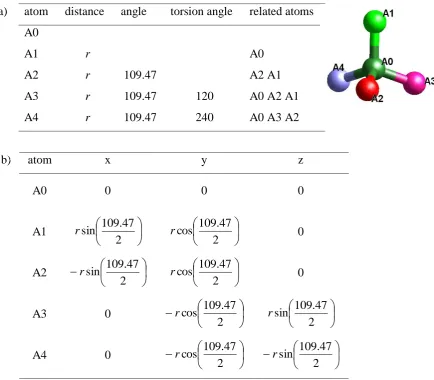
the internal parameters namely bond lengths, angles and torsion angles (Leach, 2001).

In order to generate the z-matrix one starts with one atom or pseudo atom, which is

placed in the origin of the internal rigid body coordination system. It is advantageous

to use the centre of gravity as origin of the RB, even if no atom is present, to allow for

uniform rotations. Based on the center of the RB, all atoms are placed using

interatomic distances, angles and torsion angles. In the first column of a z-matrix,

starting with the second atom, the distance to a previously defined atom is given, in

the second column, starting from the third atom, an angle between the atoms and in

the third column, starting with the fourth atom, a torsion angle with respect to

previous defined cites is given (Leach, 2001). A comparison of the two possible

descriptions of a RB for a tetrahedron is given in Table 3.1 (Dinnebier & Müller,

2012).

During a phase transition the orientation and position of a RB within a crystal

structure might change. In order to follow such changes the up to six position and

orientation parameters of the RB need to be followed within refinement of a series of

in-situ powder diffraction data. This can be performed for simple structures, though,

for more complex ones, a different approach reducing the number of parameters even

further can be beneficial. Furthermore the interatomic distances and angles within the

RB might change so that they need to be analysed as well.

In order to facilitate and enhance the analysis of rigid body rotations during a phase

transition, a symmetry adapted parameter set was developed. The new parameter set,

which is denoted as rigid body symmetry modes, combines features of rigid bodies

and symmetry modes. In this method, the orientation and position of a RB is given by

a rotational vector. In general, both, rotational and displacive vectors can be used to

describe a crystal structure, though the intrinsic tensor properties are different. An

(36)

one, which leads to different behaviour with respect to symmetry elements. However

it can be shown that intrinsic and extended rigid body rotations can be described

within traditional crystallographic space groups (Müller et al., 2013).

Table 3.1: Comparison of different RB descriptions of a tetrahedron composed of five atoms using a) z-matrix notation and b) Cartesian coordinates. The distance between two neighbouring atoms is r. The angle of 109.47° is the typical tetrahedron angle.

b) atom x y z

A0 0 0 0

A1 

     2 47 . 109 sin r       2 47 . 109 cos r 0

A2 

      2 47 . 109 sin r       2 47 . 109 cos r 0

A3 0 

      2 47 . 109 cos r       2 47 . 109 sin r

A4 0 

      2 47 . 109 cos r        2 47 . 109 sin r

3.1.3 The theory of phase transitions (Landau theory)

A phase transition within a material is characterized by a discontinuous change of at

least one material property (e.g. density, elasticity, magnetic and electric properties or

crystal structure). Throughout the work of this thesis, different structural phase

transitions with different mechanisms were studied.

a) atom distance angle torsion angle related atoms

A0

A1 r A0

A2 r 109.47 A2 A1

A3 r 109.47 120 A0 A2 A1

(37)

The type of structural change can be used to distinguish structural phase transition

into different classes. During a reconstructive phase transition, atomic bonds are

broken and/or build. The crystal structure can change completely; therefore this

process cannot be continuous. A contrast to such transitions is the displacive

transition. During a displacive phase transition, atomic positions change continuously.

A third type of transitions is the order-disorder transition, which is characterized by a

change in atomic positions between an ordered arrangement and a less ordered

arrangement.

In another classification all phase transitions, which are accompanied by a change in

the point group symmetry are called ferroic. A ferroic distortion can be further

classified as ferroelastic if it changes the shape of the unit cell in such a way as to

alter the crystal system (Wadhawan, 1982).

In 1933, Ehrenfest (Ehrenfest, 1933) developed a classification of phase transitions

which is based on the thermodynamic free energy G (also known as Gibbs energy).

Transitions which are characterized by a jump of the first derivative of the

thermodynamic free energy G are called first-order. In case of second-order

transitions, volume and entropy change continuously, though the second derivative of

the Gibbs free energy G exhibits a jump (Müller, 2012). Nowadays, phase transitions

are distinguished in discontinuous and continuous transitions, whereupon still the

phrase “first-order transition” is used for discontinuous transitions and “second-order

transition” for continuous transitions. In case of a discontinuous or hysteretic

transition, the order parameter and the entropy jump at the transition point, while in

case of a continuous transition, they change smoothly, requiring that another

thermodynamic function is discontinuous (Müller, 2012).

In order to describe phase transitions, Landau developed a phenomenological theory

(Landau, 1937). Based on the precondition that there is a group-subgroup relation

between the HS and LS structure, a thermodynamic variable needs to exist in order to

describe the thermodynamic state of the LS phase (Salje, 1990). Therefore a new

variable was introduced: the order parameter Q. The energy difference of the Gibbs

energy, which stabilises the LS phase, is thus dependent on the usual parameters

(38)

The order parameter decreases continuously to zero at a second-order phase transition,

whereas an order parameter can abruptly "jump" at a first-order transition. In case of a

temperature dependent phase transition, the order parameter Q can be modelled by an

empirical power law of the form:

 T T f

Q crit  (3.2)

where Tcrit is the transition temperature, β6 is the critical exponent, and f is a prefactor.

Typical values of β are ½ for ordinary scalar second-order transitions, or ¼ for a

transition at the tricritical point that marks the boundary between first- and

second-order transitions. Values between ¼ and ½ might be obtained for a variety of reasons

(Salje, 1990; Cowley, 1980).

The Landau critical exponent is derived by calculating the first derivative of the

Taylor series expansion of a truncated Gibbs energy with respect to the order

parameter and setting it to zero (Landau, 1937; Müller, 2012):

0    Q G

. (3.3)

This approach is correct for small values of Q (close to Tcrit), though it has proven to

be applicable in a larger range. A truncation of the Taylor series is possible, if the last

term has a positive prefactor, which guarantees that an increase in Q leads to an

increase in G (Müller, 2012).

Within the Taylor series of G (also known as Landau potential) only even power

terms are allowed as G must be positive, independent from the sign of Q, in case of a

continuous phase transition (Müller, 2012):

6 4 2 0 6 1 4 1 2 1 CQ BQ AQ G

G     . (3.4)

6_β

(39)

For temperatures above Tcrit a minimum is given for the trivial solutionQ0. Below

Tcrit a minimum will be present atQ0, so the dependence of the prefactors A, B and

C on temperature must be evaluated. The factor A is the most important one, it need

to be zero at the transition temperature Tcrit, above Tcrit it must be positive, and below

negative. The simplest solution, which fulfils the above requirements, is a linear

dependency:

) (T T_crit k

A  with k 0. (3.5)

Assuming B to beB0, C can be set to zero as its influence in this case is negligible. Under these conditions, the Landau potential is reduced to its 2nd and 4th order terms,

which is called 2-4 potential (Salje, 1990; Müller 2012):

4 2 0 4 1 2 1 BQ AQ G

G    . (3.6)

Taking the derivative leads to:

0 3      BQ AQ Q G (3.7)

and Q(ABQ2)0. (3.8)

The trivial solution is Q0for T > Tcrit. Otherwise the solution is: 2

Q B A _

 . (3.9)

Using equation (3.5) for A, the following result for T < Tcrit will be obtained:



Q 2

1

)

(T T_crit

B

k _

 or more general 2

1

) (T Tcrit

f

Q  , (3.10)

which proves that the critical exponent β = ½ for a second-order phase transition

(40)

In a similar way it can be shown that in case of a tricritical (also called “weakly”

first-order) transition a value of ¼ is obtained (Salje, 1990). In this case the same

behaviour of A is assumed, though B is assumed to be not positive, and therefore is set

to zero. This requires using the 6th order term with C > 0. The resulting potential is

denoted as 2-6 potential (Salje, 1990; Müller, 2012):

6 2 0 6 1 2 1 CQ AQ G

G    . (3.11)

As for the previous case, the derivative needs to be taken and the following equations

are obtained: 0 5      CQ AQ Q G (3.12) 0 ) (ACQ4 

Q . (3.13)

Using equation (3.5) for A, solutions of equation (3.13) are:

0



Q for T > Tcrit and

4 1

4 ₍_T _T_crit₎

C k

Q   or more general 4

1 ) (T T_crit f

Q  . (3.14)

So for a tricritical phase transition the critical exponent β is equal to ¼.

It has also been shown that non-standard critical exponents β obtained from fits over

extended temperature ranges are often due to temperature-dependent

energy-expansion coefficients of order four or higher and have nothing at all to do with

critical phenomena (Giddy et al., 1989; Radescu et al., 1995).

As Landau theory can describe ferroic phase transitions, an equation based on

equation (3.2) was used in sequential and parametric Rietveld refinements in order to

model the behaviour of parameters in dependence on an external variable.

(41)

3.2 The first-order phase transition of CsFeO2

The work presented in this chapter was published in: Melanie Müller, Robert E.

Dinnebier, Naveed Z. Ali, Branton Campbell and Martin Jansen: Direct Access to the

Order Parameter: Parameterized Symmetry Modes and Rigid Body Movements as a

Function of Temperature. Materials Science Forum (Extending the Reach of Powder

Diffraction Modelling) (2010) 651, 79-95.

Sample synthesis was performed by Naveed Zafar Ali (formerly Max Planck Institute

for Solid State Research). The synchrotron measurements were performed by Denis

Sheptyakov from Laboratory for Neutron Scattering, ETH Zürich (Switzerland) and

PSI Villigen (Switzerland).

3.2.1 Introduction

The first-order phase transition of CsFeO2 was investigated using in-situ synchrotron

powder diffraction data measured in dependence on temperature. Two alternative

approaches were used to describe the deviation of the framework crystal structure

relative to the high symmetry parent structure: symmetry modes (SM) and rigid body

(RB) parameters. In both cases, the relevant parameters were refined as a function of

temperature using the method of parametric Rietveld refinement (Müller et al., 2010).

3.2.1.1 The compound CsFeO2

CsFeO2 belongs to the group of alkali metal oxoferrats(III) with composition AFeO2.

Those compounds as well as other oxoferrates(III) of light alkali metals are

structurally closely related to the group of oxosilicates due to the predominance of

tetrahedral coordination of Fe(III) (Frisch & Röhr, 2005). Most of the alkali metal

oxoferrats(III) crystallise in structures which can be derived from a stuffed

β-cristobalite structure, so they are members of the structure family of feldspars (Nuss et

(42)

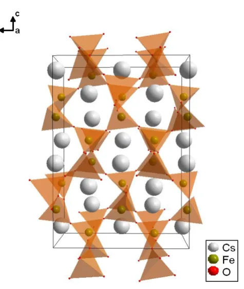
At ambient conditions, CsFeO2 crystallises in the orthorhombic space group Pbca.At

about 80°C, it undergoes a first-order phase transition to the cubic space group

m

Fd3 (Ali et al., 2010). The LS crystal structure is shown in Figure 3.1. Within the HS cubic structure the Fe-O tetrahedra are arranged in a more ordered way. The

difference between the arrangements can be seen in Figure 3.2.

(43)

Figure 3.2: Arrangement of six connected Fe-O tetrahedra within the low symmetry orthorhombic (a) and high symmetry cubic (b) structures of CsFeO2. Within the LS structure the tetrahedra are twisted with respect to each other.

3.2.2 Experimental

3.2.2.1 Material synthesis

Sample preparation was performed following the azide/nitrate route (Trinschek &

Jansen, 1999; Sofin et al., 2002) using cesium nitrate (CsNO3), cesium azide (CsN3)

and active iron oxide (Fe2O3) according to the following equation:

5 CsN3 + CsNO3 + 3Fe2O3 → 6 CsFeO2 + 8 N2 . (3.15)

The preparation process was described by Ali et al. (2010). After grinding the

appropriate amount of the starting materials (see equation (3.15)), the obtained

powder was pressed into pellets under nitrogen pressure. These pellets were dried in

vacuum at 127°C and given into a steel vessel with silver inlet under argon

atmosphere. Following a suitable temperature profile (Ali et al., 2010), a powdered

sample was obtained, which is sensitive to humidity and thus must be handled in inert

(44)

3.2.2.2 Measurement

For temperature dependent in-situ powder diffraction measurements, the material was

sealed into a Hilgenberg quartz-glass capillary with a diameter of 0.3 mm.

Measurements were performed at the Materials Sciences (MS-Powder) beamline of

the Swiss Light Source using synchrotron radiation at a wavelength of 0.49701 Å.

The powder sample was heated from 30 – 136°C with steps of 1K using a STOE

capillary furnace. The diffraction patterns were collected using a Microstrip

Mythen-II detector with an acquisition time of 40 seconds for each pattern (4 scans of 10

seconds each) in the angular range from 3.0° – 53.38° 2θ.

3.2.3 Method and Results

Two different models were used for structural description during the phase transition

from orthorhombic to cubic CsFeO2. The first approach, which was applied, is the

symmetry mode approach, which will be denoted as SM. In order to obtain the

required information to do the symmetry mode Rietveld refinements, CIFs of the HS

m

Fd3 and LS Pbca phases were subjected to the ISODISTORT software to perform an automatic symmetry mode decomposition of the low symmetry distorted structure

into modes of the high symmetry cubic parent.

The cubic phase contains in total 32 atoms in the conventional face-centred unit cell,

which do not have any general atomic coordinates, so all atoms are placed on special

Wyckoff positions. In the orthorhombic phase, however, there are 24 free atomic

coordinates. Because the symmetry mode basis is related to the traditional atomic

coordinate basis by a linear transformation, there must also be 24 displacive

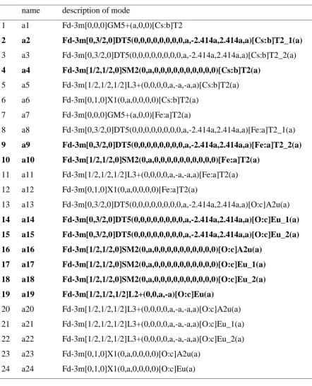
symmetry modes (Müller et al., 2010). A list of all modes is given in Table 3.2. Table

3.2 contains number, name and description of each symmetry mode. Within the mode

name the parent space group symmetry, the k-point (the point in reciprocal space that

will get intensity if the mode is activated), the space group irrep label and order

parameter direction (dictates which space group symmetry operations are preserved

(45)

the point-group symmetry (dictates which site symmetry operations are preserved by

the mode) and the order parameter branch are given (Campbell et al., 2006).

Furthermore these results are saved in form of a set of linear equations, which can be

used in Rietveld refinement.

In order to describe the phase transition the mode amplitudes of ten out of the 24

displacive symmetry modes need to be refined, while the others are set to zero. The

following modes were used in refinement (see Table 3.2): two (a2 and a4) for caesium,

two (a9 and a10) for iron and six (a14, a15, a16, a17, a18 and a19) for oxygen. The a2

-mode affects the y-coordinates of both caesium atoms, while a4 only affects the x

-coordinate of Cs2. The a9 mode influences the y-coordinate of the Fe1 and Fe2 atoms,

while the a10 mode influences only the x-coordinate of the Fe1 atom. The combination

of the oxygen modes a14 to a19 describes the rotation of the FeO4 tetrahedron, which

should not be substantially distorted (Müller et al., 2010).

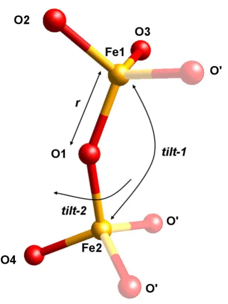
Furthermore the crystal structure of CsFeO2 was described using rigid bodies. In order

to do so, a RB which can describe the LS and HS crystal structure was developed. It is

built of two corner sharing FeO4 tetrahedra, which can be tilted with respect to each

other. The RB consists of two iron and four oxygen atoms, the other atoms, needed to

complete the tetrahedra, are generated by space group symmetry (Müller et al., 2010).

Within the RB, there are three internal degrees of freedom: two tilting angles and the

average interatomic distance r. The two tilt angles are (1) the Fe1-O1-Fe2 (tilt-1)

bond angle and (2) the O4-Fe2-O1-Fe1 torsion angle (tilt-2) between the two

tetrahedra. The RB and the corresponding tilt angles are shown in Figure 3.3. The

(46)

Table 3.2: Symmetry-adapted distortion modes available to the ferroelastic phase transition of CsFeO2 from ̅ to Pbca symmetry. The ten modes that were

actually used for Rietveld refinements appear in bold.

name description of mode

1 a1 Fd-3m[0,0,0]GM5+(a,0,0)[Cs:b]T2

2 a2 Fd-3m[0,3/2,0]DT5(0,0,0,0,0,0,0,0,a,-2.414a,2.414a,a)[Cs:b]T2_1(a)

3 a3 Fd-3m[0,3/2,0]DT5(0,0,0,0,0,0,0,0,a,-2.414a,2.414a,a)[Cs:b]T2_2(a)

4 a4 Fd-3m[1/2,1/2,0]SM2(0,a,0,0,0,0,0,0,0,0,0,0)[Cs:b]T2(a)

5 a5 Fd-3m[1/2,1/2,1/2]L3+(0,0,0,0,a,-a,-a,a)[Cs:b]T2(a)

6 a6 Fd-3m[0,1,0]X1(0,a,0,0,0,0)[Cs:b]T2(a)

7 a7 Fd-3m[0,0,0]GM5+(a,0,0)[Fe:a]T2(a)

8 a8 Fd-3m[0,3/2,0]DT5(0,0,0,0,0,0,0,0,a,-2.414a,2.414a,a)[Fe:a]T2_1(a)

9 a9 Fd-3m[0,3/2,0]DT5(0,0,0,0,0,0,0,0,a,-2.414a,2.414a,a)[Fe:a]T2_2(a)

10 a10 Fd-3m[1/2,1/2,0]SM2(0,a,0,0,0,0,0,0,0,0,0,0)[Fe:a]T2(a)

11 a11 Fd-3m[1/2,1/2,1/2]L3+(0,0,0,0,a,-a,-a,a)[Fe:a]T2(a)

12 a12 Fd-3m[0,1,0]X1(0,a,0,0,0,0)[Fe:a]T2(a)

13 a13 Fd-3m[0,3/2,0]DT5(0,0,0,0,0,0,0,0,a,-2.414a,2.414a,a)[O:c]A2u(a)

14 a14 Fd-3m[0,3/2,0]DT5(0,0,0,0,0,0,0,0,a,-2.414a,2.414a,a)[O:c]Eu_1(a)

15 a15 Fd-3m[0,3/2,0]DT5(0,0,0,0,0,0,0,0,a,-2.414a,2.414a,a)[O:c]Eu_2(a)

16 a16 Fd-3m[1/2,1/2,0]SM2(0,a,0,0,0,0,0,0,0,0,0,0)[O:c]A2u(a)

17 a17 Fd-3m[1/2,1/2,0]SM2(0,a,0,0,0,0,0,0,0,0,0,0)[O:c]Eu_1(a)

18 a18 Fd-3m[1/2,1/2,0]SM2(0,a,0,0,0,0,0,0,0,0,0,0)[O:c]Eu_2(a)

19 a19 Fd-3m[1/2,1/2,1/2]L2+(0,0,a,-a)[O:c]Eu(a)

20 a20 Fd-3m[1/2,1/2,1/2]L3+(0,0,0,0,a,-a,-a,a)[O:c]A2u(a)

21 a21 Fd-3m[1/2,1/2,1/2]L3+(0,0,0,0,a,-a,-a,a)[O:c]Eu_1(a)

22 a22 Fd-3m[1/2,1/2,1/2]L3+(0,0,0,0,a,-a,-a,a)[O:c]Eu_2(a)

23 a23 Fd-3m[0,1,0]X1(0,a,0,0,0,0)[O:c]A2u(a)

(47)

Figure 3.3: Rigid body consisting of the Fe-O double tetrahedron in CsFeO2 exhibiting three internal parameters: r, tilt-1 and tilt-2. Solid atoms are implemented into the program; semitransparent atoms are generated due to space group symmetry.

Table 3.3: Z-matrix description of the crystallographically independent atoms of the Fe2O7 rigid body. The three internal refinable parameters (tilt-1, tilt-2 and r) are displayed in bold.

atom distance angle torsion angle related atoms

O1

Fe1

O2

O3

Fe2

O4

r

109.47

tilt-1

109.47

120

180

tilt-2

O1

Fe1 O1

Fe1 O2 O1

O1 Fe1 O2

(48)

For Rietveld refinement, the orientation and position of the RB relative to the internal

coordinate system of the crystal were kept constant over the entire temperature range

of investigation and only the three internal degrees of freedom were subjected to

refinement. As the two caesium atoms in the voids of the framework are independent

of the RB, their crystallographically relevant atomic coordinates were refined

separately (Müller et al., 2010).

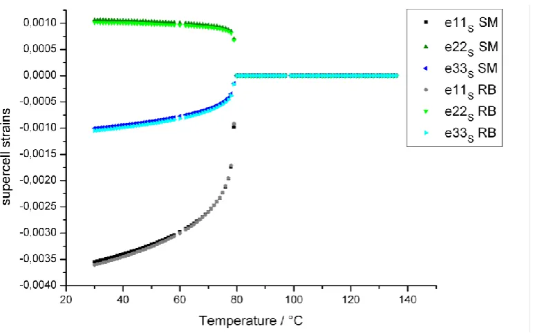
The behaviour of the lattice parameters in dependence on temperature was described

using lattice strain. Strain is a symmetric second rank tensor which is represented by a

33 matrix. In case of orthorhombic symmetry (actual supercell) it reduces to a diagonal matrix with the following diagonal elements:

⁄√ (3.16)

√ (3.17)

(3.18)

with the lattice parameters of the supercell as, bs, cs and the isothermal lattice

parameters as0, bs0 and cs0. The isothermal lattice parameters can be given as well in

dependence on the isothermal lattice parameters of the cubic parent cell ap0.

The same description can be used in dependence on the cubic parent cell. In this case,

strain is represented by a diagonal matrix with e11p e22p e33p and

0

13 23

12p e p e p 

e (Müller et al., 2010).

Upon formation of the ferroelastic strain, the parent cell becomes a pseudo-cubic

monoclinic cell defined by three independent order parameters that we will denote by



 , where  indicates one of three strain mode irreps: ₁, ₃ and ₅. The ₁ mode

causes a thermal expansion. The ₃ mode affects the ratio of the lattice parameters a

and b with respect to the lattice parameter c. And the ₅ mode results in a monoclinic

shear that changes the parent lattice angle γ and gives rise to a non-zero e12 strain

(49)

In the coordinate system of the parent cell, the relationship

Advances in the modelling of in-situ powder diffraction data