R E S E A R C H
Open Access
Approximate solutions for MHD squeezing
fluid flow by a novel method
Mustafa Inc
1and Ali Akgül
2,3**Correspondence:
[email protected]; [email protected]
2Department of Mathematics,
Education Faculty, Dicle University, Diyarbakır, 21280, Turkey
3Department of Mathematics, Texas
A&M University-Kingsville, Kingsville, USA
Full list of author information is available at the end of the article
Abstract
In this paper, a steady axisymmetric MHD flow of two-dimensional incompressible fluids has been investigated. The reproducing kernel Hilbert space method (RKHSM) has been implemented to obtain a solution of the reduced fourth-order nonlinear boundary value problem. Numerical results have been compared with the results obtained by the Runge-Kutta method (RK-4) and optimal homotopy asymptotic method (OHAM).
MSC: 46E22; 35A24
Keywords: reproducing kernel method; series solutions; squeezing fluid flow; magnetohydrodynamics; reproducing kernel space
1 Introduction
Squeezing flows have many applications in food industry, principally in chemical engi-neering [–]. Some practical examples of squeezing flow include polymer processing, compression and injection molding. Grimm [] studied numerically the thin Newtonian liquids films being squeezed between two plates. Squeezing flow coupled with magnetic field is widely applied to bearing with liquid-metal lubrication [, –].
In this paper, we use RKHSM to study the squeezing MHD fluid flow between two in-finite planar plates. This problem has been solved by RKHSM and for comparison it has been compared with the OHAM and numerically with the RK- by using Maple .
The RKHSM, which accurately computes the series solution, is of great interest to ap-plied sciences. The method provides the solution in a rapidly convergent series with com-ponents that can be elegantly computed. The efficiency of the method was used by many authors to investigate several scientific applications. Geng and Cui [] and Zhouet al.[] applied the RKHSM to handle the second-order boundary value problems. Yao and Cui [] and Wanget al.[] investigated a class of singular boundary value problems by this method and the obtained results were good. Wang and Chao [], Li and Cui [], Zhou and Cui [] independently employed the RKSHSM to variable-coefficient partial differ-ential equations. Du and Cui [] investigated the approximate solution of the forced Duff-ing equation with integral boundary conditions by combinDuff-ing the homotopy perturbation method and the RKM. Lv and Cui [] presented a new algorithm to solve linear fifth-order boundary value problems. Cui and Du [] obtained the representation of the exact solu-tion for the nonlinear Volterra-Fredholm integral equasolu-tions by using the RKHSM. Wu and Li [] applied iterative RKHSM to obtain the analytical approximate solution of a
linear oscillator with discontinuities. For more details about RKHSM and the modified forms and its effectiveness, see [–] and the references therein.
The paper is organized as follows. We give the problem formulation in Section . Sec-tion introduces several reproducing kernel spaces. A bounded linear operator is pre-sented in Section . In Section , we provide the main results, the exact and approximate solutions. An iterative method is developed for the kind of problems in the reproduc-ing kernel space. We prove that the approximate solution converges to the exact solution uniformly. Some numerical experiments are illustrated in Section . There are some con-clusions in the last section.
2 Problem formulation
Consider a squeezing flow of an incompressible Newtonian fluid in the presence of a mag-netic field of a constant densityρand viscosityμsqueezed between two large planar par-allel plates separated by a small distance Hand the plates approaching each other with a low constant velocityV, as illustrated in Figure , and the flow can be assumed to quasi-steady [–, ]. The Navier-Stokes equations [, ] governing such flow in the presence of magnetic field, when inertial terms are retained in the flow, are given as []
∇V·u= (.)
and
ρ
∂u
∂t + (u· ∇)u
=∇ ·T+J×B+ρf, (.)
whereuis the velocity vector, ∇ denotes the material time derivative,T is the Cauchy stress tensor,
T= –pI+μA
and
A=∇u+uT,
Jis the electric current density,Bis the total magnetic field and
B=B+b,
B represents the imposed magnetic field andbdenotes the induced magnetic field. In
the absence of displacement currents, the modified Ohm law and Maxwell’s equations (see [] and the references therein) are given by []
J=σ[E+u×B] (.)
and
divB= , ∇ ×B=μmJ, curlE=
∂B
∂t, (.)
in whichσ is the electrical conductivity, E is the electric field andμm is the magnetic permeability.
The following assumptions are needed [].
(a) The densityρ, magnetic permeabilityμmand electric field conductivityσare
assumed to be constant throughout the flow field region.
(b) The electrical conductivityσof the fluid is considered to be finite.
(c) Total magnetic fieldBis perpendicular to the velocity fieldV and the induced magnetic fieldbis negligible compared with the applied magnetic fieldBso that
the magnetic Reynolds number is small (see [] and the references therein). (d) We assume a situation where no energy is added or extracted from the fluid by the
electric field, which implies that there is no electric field present in the fluid flow region.
Under these assumptions, the magnetohydrodynamic force involved in Eq. (.) can be put into the form
J×B= –σBu. (.)
An axisymmetric flow in cylindrical coordinatesr, θ, z withz-axis perpendicular to plates andz=±Hat the plates. Since we have axial symmetry,uis represented by
u=ur(r,z), ,uz(r,z)
,
when body forces are negligible, Navier-Stokes Eqs. (.)-(.) in cylindrical coordinates, where there is no tangential velocity (uθ= ), are given as []
ρ
ur
∂ur
∂r +uz ∂ur
∂z
= –∂p
∂r +
∂u
r
∂r +
r ∂ur
∂r – ur
r + ∂u
r
∂z
+σBu (.)
and
ρ
uz
∂uz
∂r +uz ∂uz
∂z
= –∂p
∂r +
∂u
z
∂r +
r ∂uz
∂r + ∂u
z
∂z
wherepis the pressure, and the equation of continuity is given by []
r ∂ ∂r(rur) +
∂uz
∂z = . (.)
The boundary conditions require
ur= , uz= –V atz=H,
∂ur
∂z = , uz= atz= .
(.)
Let us introduce the axisymmetric Stokes stream functionas
ur=
r ∂
∂z, uz= –
r ∂
∂r. (.)
The continuity equation is satisfied using Eq. (.). Substituting Eqs. (.)-(.) and Eq. (.) into Eqs. (.)-(.), we obtain
–ρ
r ∂
∂rE
= –∂p ∂r+
μ r
∂E ∂z –
σB r
∂
∂z (.)
and
–ρ
r ∂
∂zE
= –∂p ∂z +
μ r
∂E
∂r . (.)
Eliminating the pressure from Eqs. (.) and (.) by the integrability condition, we get the compatibility equation as []
–ρ
∂(,E
r ) ∂(r,z)
=μ
rE
–σB r
∂
∂z, (.)
where
E= ∂
∂r –
r ∂ ∂r+
∂ ∂z.
The stream function can be expressed as [, ]
(r,z) =rF(z). (.)
In view of Eq. (.), the compatibility equation (.) and the boundary conditions (.) take the form
F(iv)(z) –σB
r F
(z) + ρ μF(z)F
(z) = , (.)
subject to
F() = , F() = ,
F(H) =V
, F
Non-dimensional parameters are given as []
F∗= F
V, z
∗= z
H, Re=
ρHV
μ , m=BH
σ μ.
For simplicity omitting the∗, the boundary value problem (.)-(.) becomes []
F(iv)(z) –mF(z) +ReF(z)F(z) = , (.)
with the boundary conditions
F() = , F() = ,
F() = , F() = ,
(.)
whereReis the Reynolds number andmis the Hartmann number.
3 Reproducing kernel spaces
In this section, we define some useful reproducing kernel spaces.
Definition .(Reproducing kernel) Let Ebe a nonempty abstract set. A functionK :
E×E−→Cis a reproducing kernel of the Hilbert spaceHif and only if
∀t∈E, K(·,t)∈H,
∀t∈E,∀ϕ∈H, ϕ(·),K(·,t) =ϕ(t). (.)
The last condition is called ‘the reproducing property’: the value of the functionϕat the pointtis reproduced by the inner product ofϕwithK(·,t).
Definition . We define the spaceW
[, ] by
W[, ] = u|u,u
,u,u,u()are absolutely continuous in [, ],
u()∈L[, ],x∈[, ],u() =u() =u() =u() =
.
The fifth derivative ofuexists almost everywhere sinceu()is absolutely continuous. The
inner product and the norm inW
[, ] are defined respectively by
u,vW =
i=
u(i)()v(i)() +
u()(x)v()(x)dx, u,v∈W[, ]
and
uW =
u,u
W, u∈W
[, ].
The spaceW
[, ] is a reproducing kernel space,i.e., for each fixedy∈[, ] and any u∈W
[, ], there exists a functionRysuch that
Definition . We define the spaceW [, ] by
W[, ] = u|u,u
,u,uare absolutely continuous in [, ],
u()∈L[, ],x∈[, ]
.
The fourth derivative ofuexists almost everywhere sinceu() is absolutely continuous.
The inner product and the norm inW
[, ] are defined respectively by
u,vW =
i=
u(i)()v(i)() +
u()(x)v()(x)dx, u,v∈W[, ]
and
uW =
u,u
W, u∈W
[, ].
The spaceW
[, ] is a reproducing kernel space,i.e., for each fixedy∈[, ] and any u∈W[, ], there exists a functionrysuch that
u=u,ryW .
Theorem . The space W[, ]is a reproducing kernel Hilbert space whose reproducing kernel function is given by
Ry(x) =
i=ci(y)xi–, x≤y,
i=di(y)xi–, x>y,
where ci(y)and di(y)can be obtained easily by using Mapleand the proof of Theorem.
is given in Appendix.
Remark . The reproducing kernel functionryofW[, ] is given as
ry(x) =
+xy+ y
x+ y
x+ y
x– y
x+ yx
– ,x
, x≤y,
+yx+yx+ yx+ xy– xy+ xy–, y, x>y.
This can be proved easily as the proof of Theorem ..
4 Bounded linear operator inW25[0, 1]
In this section, the solution of Eq. (.) is given in the reproducing kernel spaceW[, ]. On defining the linear operatorL:W
[, ]→W[, ] as
Lu=u()(x) +Ree x
e
x– x+ xu()(x) –mu(x) +Ree x
e
x+ x– x– u(x).
Model problem (.)-(.) changes the following problem:
Lu=M(x,u,u()), x∈[, ],
where
F(x) =u(x) +e x
e
x– x+ x
and
Mx,u,u()= –Reu()(x)u(x) –Re
ex
e
x– x+ xx+ x– x–
–e x
e
x+ x+ x– +me
x
e
x+ x– x.
Theorem . The operator L defined by(.)is a bounded linear operator.
Proof We only need to prove
LuW
≤PLu
W ,
wherePis a positive constant. By Definition ., we have
uW
=u,u W = i=
u(i)()+
u()(x)dx, u∈W[, ],
and
LuW
=Lu,LuW =
(Lu)()+(Lu)()+(Lu)()
+(Lu)()()+
(Lu)()(x)dx.
By the reproducing property, we have
u(x) =u,Rx W ,
and
(Lu)(x) =u, (LRx)
W, (Lu)
(x) =u, (LR
x)
W,
(Lu)(x) =u, (LRx)
W, (Lu)
()(x) =u, (LR
x)()
W,
(Lu)()(x) =u, (LRx)()
W.
Therefore, by the Cauchy-Schwarz inequality, we get
(Lu)(x)≤ uW
LRxW=auW (wherea> is a positive constant),
(Lu)(x)≤ uW
(LRx)W
=auW
(wherea> is a positive constant),
(Lu)(x)≤ uW (LRx)
W=auW (wherea> is a positive constant),
(Lu)()(x)≤ uW (LRx)
()
W=auW
Thus
(Lu)()+(Lu)()+(Lu)()+(Lu)()()≤a+a+a+auW .
Since
(Lu)()=u, (LRx)()
W,
then
(Lu)()≤ uW (LRx)
()
W=auW
(wherea> is a positive constant).
Therefore, we have
(Lu)()≤auW
and
(Lu)()(x)dx≤auW ,
that is,
LuW =
(Lu)()+(Lu)()+(Lu)()+(Lu)()()+
(Lu)()(x)dx
≤a+a+a+a+au
W=Pu
W ,
whereP= (a+a+a+a+a) > is a positive constant. This completes the proof.
5 Analysis of the solution of (2.17)-(2.18)
Let{xi}∞i=be any dense set in [, ] andx(y) =L∗rx(y), whereL∗is the adjoint operator of
Landrxis given by Remark .. Furthermore
i(x)def=xi(x) =L∗rxi(x).
Lemma . {i(x)}∞i=is a complete system of W[, ].
Proof Foru∈W
[, ], let
u,i = (i= , , . . .),
that is,
u,L∗rxi
= (Lu)(xi) = .
Note that{xi}∞i= is the dense set in [, ]. Therefore (Lu)(x) = . Assume that (.) has a
unique solution. ThenLis one-to-one onW
[, ] and thusu(x) = . This completes the
Lemma . The following formula holds:
i(x) =
LηRx(η)
(xi),
where the subscriptηof the operator Lηindicates that the operator L applies to a function ofη.
Proof
i(x) =
i(ξ),Rx(ξ)
W[,]
=L∗rxi(ξ),Rx(ξ)
W[,]
=(rxi)(ξ),
LηRx(η)
(ξ)W [,]
=LηRx(η)
(xi).
This completes the proof.
Remark . The orthonormal system {i(x)}∞i= of W[, ] can be derived from the
Gram-Schmidt orthogonalization process of{i(x)}∞i=as
i(x) = i
k=
βikk(x) (βii> ,i= , , . . .), (.)
whereβikare orthogonal coefficients.
In the following, we give the representation of the exact solution of Eq. (.) in the reproducing kernel spaceW
[, ].
Theorem . If u is the exact solution of(.),then
u= ∞ i= i k= βikM
xk,u(xk),u()(xk)
i(x),
where{xi}∞i=is a dense set in[, ].
Proof From (.) and the uniqueness of solution of (.), we have
u=
∞
i=
u,i Wi=
∞ i= i k= βik u,L∗rxk
Wi
= ∞ i= i k=
βikLu,rxk W i=
∞ i= i k= βik
Mx,u,u(),rxk
Wi
= ∞ i= i k= βikM
xk,u(xk),u()(xk)
i(x).
Now the approximate solutionuncan be obtained by truncating then-term of the exact solutionuas
un= n
i=
i
k= βikM
xk,u(xk),u()(xk)
i(x).
Lemma .([]) Assume that u is the solution of(.)and rnis the error between the
approximate solution unand the exact solution u.Then the error sequence rnis monotone
decreasing in the sense of · W
andrn(x)W→.
6 Numerical results
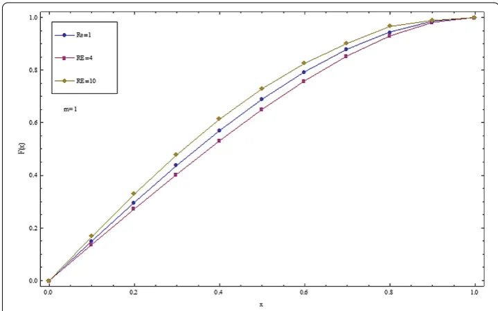
In this section, comparisons of results are made through different Reynolds numbersRe and magnetic field effectm. All computations are performed by Maple . Figure . shows comparisons ofF(z) for a fixed Reynolds number with increasing magnetic field effect
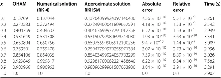
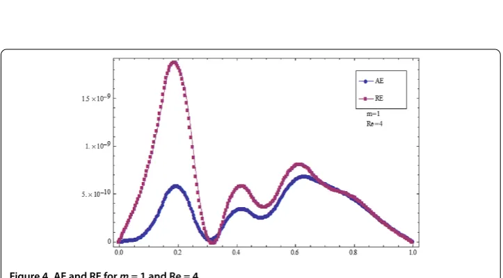
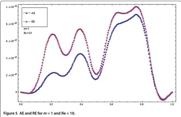
m= , , , . From this figure, the velocity decreases due to an increase inm. Figure . shows comparisons ofF(z) for a fixed magnetic fieldm= with increasing Reynolds num-bersRe= , , . It is observed that much increase in Reynolds numbers affects the results. The RKHSM does not require discretization of the variables,i.e., time and space, it is not affected by computation round of errors and one is not faced with necessity of large com-puter memory and time. The accuracy of the RKHSM for the MHD squeezing fluid flow is controllable and absolute errors are small with present choice ofx(see Tables - and Figures -). The numerical results we obtained justify the advantage of this methodology. Generally it is not possible to find the exact solution of these problems.
Table 1 Numerical results atm= 1 and Re = 1
x OHAM Numerical solution (RK-4)
Approximate solution RKHSM
Absolute error
Relative error
Time (s)
0.1 0.150265 0.150294 0.15029400074386619072 7.43×10⁻¹⁰ 4.94×10⁻⁹ 2.948
0.2 0.297424 0.297481 0.29748099943286204844 5.67×10⁻¹⁰ 1.9×10⁻⁹ 2.980
0.3 0.438387 0.438467 0.43846699936146542481 6.38×10⁻¹⁰ 1.45×10⁻⁹ 2.870
0.4 0.570093 0.570189 0.57018899983086605298 1.69×10⁻¹⁰ 2.96×10⁻¹⁰ 2.792
0.5 0.68952 0.689624 0.68962399932753349664 6.72×10⁻¹⁰ 9.75×10⁻¹⁰ 2.824
0.6 0.793695 0.793796 0.79379600052975674440 5.29×10⁻¹⁰ 6.67×10⁻¹⁰ 2.902
0.7 0.879695 0.879779 0.87977900034152532706 3.41×10⁻¹⁰ 3.88×10⁻¹⁰ 2.964
0.8 0.944641 0.944696 0.94469600021478585921 2.14×10⁻¹⁰ 2.27×10⁻¹⁰ 2.808
0.9 0.985687 0.985707 0.98570699945336089741 5.46×10⁻¹⁰ 5.54×10⁻¹⁰ 2.761
1.0 1.0 1.0 1.0 0.0 0.0 2.902
Table 2 Numerical results atm= 3 and Re = 1
x OHAM Numerical solution (RK-4)
Approximate solution RKHSM
Absolute error
Relative error
Time (s)
0.1 0.13709 0.137044 0.13704399924397146430 7.56×10⁻¹⁰ 5.51×10⁻⁹ 3.261
0.2 0.272583 0.272494 0.27249400041809657591 4.18×10⁻¹⁰ 1.53×10⁻⁹ 3.542
0.3 0.404759 0.404637 0.40463699937791012358 6.22×10⁻¹⁰ 1.53×10⁻⁹ 2.949
0.4 0.531649 0.531508 0.53150799980699743080 1.93×10⁻¹⁰ 3.63×10⁻¹⁰ 3.541
0.5 0.650894 0.650756 0.65075599905912100256 9.4×10⁻¹⁰ 1.44×10⁻⁹ 3.089
0.6 0.759591 0.759478 0.75947799979255971384 2.07×10⁻¹⁰ 2.73×10⁻¹⁰ 2.996
0.7 0.854106 0.854035 0.85403499924057783299 7.59×10⁻¹⁰ 8.89×10⁻¹⁰ 3.026
0.8 0.929845 0.929817 0.92981700082221438640 8.22×10⁻¹⁰ 8.84×10⁻¹⁰ 7.582
0.9 0.980966 0.980963 0.98096299961587653980 3.84×10⁻¹⁰ 3.91×10⁻¹⁰ 3.291
Table 3 Numerical results atm= 8 and Re = 1
x OHAM Numerical solution (RK-4)
Approximate solution RKHSM
Absolute error
Relative error
Time (s)
0.1 0.11507 0.114976 0.11497599095960418967 9.04×10⁻⁹ 7.86×10⁻⁸ 4.290 0.2 0.230068 0.229882 0.22988199268533318687 7.31×10⁻⁹ 3.18×10⁻⁸ 4.134 0.3 0.344866 0.344604 0.34460400584434350472 5.84×10⁻⁹ 1.69×10⁻⁸ 4.477
0.4 0.459205 0.458904 0.45890399132822355411 8.67×10⁻⁹ 1.88×10⁻⁸ 4.275
0.5 0.572545 0.572276 0.5722759999680104400 3.19×10⁻¹¹ 5.58×10⁻¹¹ 3.931
0.6 0.683769 0.683628 0.68362799155831029523 8.44×10⁻⁹ 1.23×10⁻⁸ 4.556
0.7 0.790543 0.790607 0.79060700783664672119 7.83×10⁻⁹ 9.91×10⁻⁹ 4.461
0.8 0.887936 0.888173 0.88817300466724146312 4.66×10⁻⁹ 5.25×10⁻⁹ 3.885
0.9 0.965381 0.965578 0.96557800220185786369 2.2×10⁻⁹ 2.28×10⁻⁹ 5.007
1.0 1.0 1.0 1.0 0.0 0.0 2.902
Table 4 Numerical results atm= 20 and Re = 1
x OHAM Numerical solution (RK-4)
Approximate solution RKHSM
Absolute error
Relative error
Time (s)
0.1 0.105312 0.105391 0.10539098947593257979 1.05×10⁻⁸ 9.98×10⁻⁸ 4.134
0.2 0.210625 0.210782 0.2107819933190829 6.68×10⁻⁹ 3.16×10⁻⁸ 5.101
0.3 0.315938 0.316173 0.3161729190893567630 8.09×10⁻⁸ 2.55×10⁻⁷ 3.010
0.4 0.421249 0.421563 0.4215629919618786430 8.03×10⁻⁹ 1.9×10⁻⁸ 3.198
0.5 0.526551 0.526952 0.5269519479728988 5.2×10⁻⁸ 9.87×10⁻⁸ 3.042
0.6 0.631824 0.632324 0.632323981769674315 1.82×10⁻⁸ 2.88×10⁻⁸ 3.074
0.7 0.736971 0.737586 0.7375860570172070642 5.7×10⁻⁸ 7.73×10⁻⁸ 3.089
0.8 0.841352 0.842051 0.84205103495023398982 3.49×10⁻⁸ 4.15×10⁻⁸ 3.073
0.9 0.94035 0.940861 0.94086101815219431313 1.81×10⁻⁸ 1.92×10⁻⁸ 3.135
1.0 1.0 1.0 1.0 0.0 0.0 2.902
Table 5 Numerical results atm= 1 and Re = 4
x OHAM Numerical solution (RK-4)
Approximate solution RKHSM
Absolute error
Relative error
Time (s)
0.1 0.156218 0.158104 0.15810400012535311729 1.25×10⁻¹⁰ 7.92×10⁻¹⁰ 5.304
0.2 0.308363 0.311962 0.31196200057873017887 5.78×10⁻¹⁰ 1.85×10⁻⁹ 7.332
0.3 0.452557 0.457539 0.45753900003164153289 3.16×10⁻¹¹ 6.91×10⁻¹¹ 5.913 0.4 0.585287 0.591193 0.59119300033029000468 3.3×10⁻¹⁰ 5.58×10⁻¹⁰ 6.272 0.5 0.703518 0.709771 0.70977100026331200670 2.63×10⁻¹⁰ 3.7×10⁻¹⁰ 5.757 0.6 0.804726 0.810642 0.81064200064720692438 6.47×10⁻¹⁰ 7.98×10⁻¹⁰ 6.256 0.7 0.886838 0.891666 0.89166599939606220359 6.03×10⁻¹⁰ 6.03×10⁻¹⁰ 6.396
0.8 0.948051 0.95112 0.95112000044608660232 4.46×10⁻¹⁰ 4.69×10⁻¹⁰ 5.101
0.9 0.986529 0.987612 0.98761199979328069240 2.06×10⁻¹⁰ 2.09×10⁻¹⁰ 5.616
1.0 1.0 1.0 1.0 0.0 0.0 2.902
Table 6 Numerical results atm= 1 and Re = 10
x OHAM Numerical solution (RK-4)
Approximate solution RKHSM
Absolute error
Relative error
Time (s)
0.1 0.175911 0.167616 0.1676160001397322991 1.39×10⁻¹⁰ 8.33×10⁻¹⁰ 5.569
0.2 0.344336 0.329031 0.32903100221406728329 2.21×10⁻⁹ 6.72×10⁻⁹ 6.365
0.3 0.498671 0.478907 0.47890699791462877619 2.08×10⁻⁹ 4.35×10⁻⁹ 7.378
0.4 0.633941 0.613252 0.61325199550552162812 4.49×10⁻⁹ 7.32×10⁻⁹ 7.254
0.5 0.747277 0.729428 0.72942799845508679063 1.54×10⁻⁹ 2.11×10⁻⁹ 6.271
0.6 0.838004 0.825843 0.82584300690485584332 6.9×10⁻⁹ 8.36×10⁻⁹ 7.425
0.7 0.907244 0.901576 0.90157600840425340903 8.4×10⁻⁹ 9.32×10⁻⁹ 6.162
0.8 0.956954 0.901576 0.90157518382496567601 8.16×10⁻⁷ 9.05×10⁻⁷ 7.410
0.9 0.988387 0.988978 0.98897799997420425356 2.57×10⁻¹¹ 2.6×10⁻¹¹ 7.910
Figure 2 Comparison RKHSM, OHAM and RK-4 solutions form= Re = 1.
Figure 3 Comparison RKHSM, OHAM and RK-4 solutions form= 3 and Re = 1.
Figure 5 AE and RE form= 1 and Re = 10.
Figure 6 Comparison of squeezing flow for a fixed Reynolds number Re = 1 and increasing magnetic field effectm= 1, 3, 8, 20.
7 Conclusion
In this paper, we introduced an algorithm for solving the MHD squeezing fluid flow. We
applied a new powerful method RKHSM to the reduced nonlinear boundary value prob-lem. The approximate solution obtained by the present method is uniformly convergent. Clearly, the series solution methodology can be applied to much more complicated
nonlin-ear differential equations and boundary value problems. However, if the problem becomes nonlinear, then the RKHSM does not require discretization or perturbation and it does not make closure approximation. Results of numerical examples show that the present
Figure 7 Comparison of squeezing flow for a fixed magnetic field effectm= 1 and increasing Reynolds numbers Re = 1, 4, 10.
Appendix
Proof of Theorem. Letu∈W
[, ]. By Definition . we have
u,Ry W
=
i=
u(i)()R(yi)() +
u()(x)R()y (x)dx. (A.)
Through several integrations by parts for (A.), we have
u,Ry W
=
i=
u(i)()R(yi)() – (–)(–i)R(–y i)()
+
i=
(–)(–i)u(i)()R(–y i)()–
u(x)R()y (x)dx. (A.)
Note the property of the reproducing kernel
u,Ry W=u(y).
Now, if
⎧ ⎪ ⎪ ⎪ ⎪ ⎪ ⎪ ⎪ ⎪ ⎨ ⎪ ⎪ ⎪ ⎪ ⎪ ⎪ ⎪ ⎪ ⎩
Ry() +R()y () = ,
R()y () +R()y () = ,
R()y () –R()y () = ,
R()y () = ,
R()y () = ,
R()y () = ,
then (A.) implies that
R()y (x) = –δ(x–y),
whenx=y
R()y (x) = ,
and therefore
Ry(x) =
i=ci(y)xi–, x≤y,
i=di(y)xi–, x>y.
Since
R()y (x) =δ(x–y),
we have
Ry(k+)(y) =Ry(k–)(y), k= , , , , , , , , , (A.)
and
R()y+(y) –R()y–(y) = –. (A.)
SinceRy(x)∈W[, ], it follows that
Ry() = , Ry() = , Ry() = , Ry() = . (A.)
From (A.)-(A.), the unknown coefficientsci(y) anddi(y) (i= , , . . . , ) can be obtained.
This completes the proof.
Competing interests
The authors declare that they do not have any competing or conflict of interests.
Authors’ contributions
Both authors contributed equally to this paper.
Author details
1Department of Mathematics, Science Faculty, Fırat University, Elazı ˘g, 23119, Turkey.2Department of Mathematics,
Education Faculty, Dicle University, Diyarbakır, 21280, Turkey.3Department of Mathematics, Texas A&M
University-Kingsville, Kingsville, USA.
Acknowledgements
We presented this paper in the International Symposium on Biomathematics and Ecology Education Research in 2013. We would like to thank the organizers of this conference and the reviewers for their kind and helpful comments on this paper. Ali Akgül gratefully acknowledge that this paper was partially supported by the Dicle University and the Firat University. This paper is a part of PhD thesis of Ali Akgül.
References
1. Papanastasiou, TC, Georgiou, GC, Alexandrou, AN: Viscous Fluid Flow. CRC Press, Boca Raton (1994)
2. Stefa Hughes, WF, Elco, RA: Magnetohydrodynamic lubrication flow between parallel rotating disks. J. Fluid Mech.13, 21-32 (1962)
3. Ghori, QK, Ahmed, M, Siddiqui, AM: Application of homotopy perturbation method to squeezing flow of a Newtonian fluid. Int. J. Nonlinear Sci. Numer. Simul.8, 179-184 (2007)
4. Ran, XJ, Zhu, QY, Li, Y: An explicit series solution of the squeezing flow between two infinite plates by means of the homotopy analysis method. Commun. Nonlinear Sci. Numer. Simul.14, 119-132 (2009)
5. Grimm, RG: Squeezing flows of Newtonian liquid films an analysis include the fluid inertia. Appl. Sci. Res.32, 149-166 (1976)
6. Kamiyama, S: Inertia effects in MHD hydrostatic thrust bearing. J. Lubr. Technol.91, 589-596 (1969) 7. Hamza, EA: The magnetohydrodynamic squeeze film. J. Tribol.110, 375-377 (1988)
8. Bhattacharya, S, Pal, A: Unsteady MHD squeezing flow between two parallel rotating discs. Mech. Res. Commun.24, 615-623 (1997)
9. Geng, F, Cui, M: Solving a nonlinear system of second order boundary value problems. J. Math. Anal. Appl.327, 1167-1181 (2007)
10. Zhou, Y, Lin, Y, Cui, M: An efficient computational method for second order boundary value problems of nonlinear differential equations. Appl. Math. Comput.194, 357-365 (2007)
11. Yao, H, Cui, M: A new algorithm for a class of singular boundary value problems. Appl. Math. Comput.186, 1183-1191 (2007)
12. Wang, W, Cui, M, Han, B: A new method for solving a class of singular two-point boundary value problems. Appl. Math. Comput.206, 721-727 (2008)
13. Wang, YL, Chao, L: Using reproducing kernel for solving a class of partial differential equation with variable-coefficients. Appl. Math. Mech.29, 129-137 (2008)
14. Li, F, Cui, M: A best approximation for the solution of one-dimensional variable-coefficient Burgers’ equation. Numer. Methods Partial Differ. Equ.25, 1353-1365 (2009)
15. Zhou, S, Cui, M: Approximate solution for a variable-coefficient semilinear heat equation with nonlocal boundary conditions. Int. J. Comput. Math.86, 2248-2258 (2009)
16. Du, J, Cui, M: Solving the forced Duffing equations with integral boundary conditions in the reproducing kernel space. Int. J. Comput. Math.87, 2088-2100 (2010)
17. Lv, X, Cui, M: An efficient computational method for linear fifth-order two-point boundary value problems. J. Comput. Appl. Math.234, 1551-1558 (2010)
18. Du, J, Cui, M: Constructive proof of existence for a class of fourth-order nonlinear BVPs. Comput. Math. Appl.59, 903-911 (2010)
19. Wu, BY, Li, XY: Iterative reproducing kernel method for nonlinear oscillator with discontinuity. Appl. Math. Lett.23, 1301-1304 (2010)
20. Cui, M, Lin, Y: Nonlinear Numerical Analysis in the Reproducing Kernel Spaces. Nova Science Publishers, New York (2009)
21. Lü, X, Cui, M: Analytic solutions to a class of nonlinear infinite-delay-differential equations. J. Math. Anal. Appl.343, 724-732 (2008)
22. Jiang, W, Cui, M: Constructive proof for existence of nonlinear two-point boundary value problems. Appl. Math. Comput.215, 1937-1948 (2009)
23. Cui, M, Du, H: Representation of exact solution for the nonlinear Volterra-Fredholm integral equations. Appl. Math. Comput.182, 1795-1802 (2006)
24. Jiang, W, Lin, Y: Representation of exact solution for the time-fractional telegraph equation in the reproducing kernel space. Commun. Nonlinear Sci. Numer. Simul.16, 3639-3645 (2011)
25. Lin, Y, Cui, M: A numerical solution to nonlinear multi-point boundary-value problems in the reproducing kernel space. Math. Methods Appl. Sci.34, 44-47 (2011)
26. Mohammadi, M, Mokhtari, R: Solving the generalized regularized long wave equation on the basis of a reproducing kernel space. J. Comput. Appl. Math.235, 4003-4014 (2011)
27. Wu, BY, Li, XY: A new algorithm for a class of linear nonlocal boundary value problems based on the reproducing kernel method. Appl. Math. Lett.24, 156-159 (2011)
28. Yao, H, Lin, Y: New algorithm for solving a nonlinear hyperbolic telegraph equation with an integral condition. Int. J. Numer. Methods Biomed. Eng.27, 1558-1568 (2011)
29. Inc, M, Akgül, A: The reproducing kernel Hilbert space method for solving Troesch’s problem. J. Assoc. Arab Univ. Basic. Appl. Sci.14, 19-27 (2013)
30. Inc, M, Akgül, A, Geng, F: Reproducing kernel Hilbert space method for solving Bratu’s problem. Bul. Malays. Math. Sci. Soc. (in press)
31. Inc, M, Akgül, A, Kilicman, A: Explicit solution of telegraph equation based on reproducing kernel method. J. Funct. Spaces Appl.2012, Article ID 984682 (2012)
32. Inc, M, Akgül, A, Kilicman, A: A new application of the reproducing kernel Hilbert space method to solve MHD Jeffery-Hamel flows problem in non-parallel walls. Abstr. Appl. Anal.2013, Article ID 239454 (2013)
33. Inc, M, Akgül, A, Kilicman, A: On solving KdV equation using reproducing kernel Hilbert space method. Abstr. Appl. Anal.2013, Article ID 578942 (2013)
34. Inc, M, Akgül, A, Kilicman, A: Numerical solutions of the second-order one-dimensional telegraph equation based on reproducing kernel Hilbert space method. Abstr. Appl. Anal.2013, Article ID 768963 (2013)
35. Akram, G, Rehman, HU: Numerical solution of eighth order boundary value problems in reproducing Kernel space. Numer. Algorithms62(3), 527-540 (2013)
36. Wenyan, W, Bo, H, Masahiro, Y: Inverse heat problem of determining time-dependent source parameter in reproducing kernel space. Nonlinear Anal., Real World Appl.14(1), 875-887 (2013)
38. Islam, S, Ullah, M, Zaman, G, Idrees, M: Approximate solutions to MHD squeezing fluid flow. J. Appl. Math. Inform. 29(5-6), 1081-1096 (2011)
39. Idrees, M, Islam, S, Haq, S, Islam, S: Application of the optimal homotopy asymptotic method to squeezing flow. Comput. Math. Appl.59, 3858-3866 (2010)
40. Mohyuddin, MR, Gotz, T: Resonance behavior of viscoelastic fluid in Poiseuille flow in the presence of a transversal magnetic field. Int. J. Numer. Methods Fluids49, 837-847 (2005)
10.1186/1687-2770-2014-18
![Figure 1 A steady squeezing axisymmetric fluid flow between two parallel plates [38].](https://thumb-us.123doks.com/thumbv2/123dok_us/506940.2049943/2.595.116.479.495.712/figure-steady-squeezing-axisymmetric-uid-ow-parallel-plates.webp)