Novel Methods based on the Fusion of Multisensor Remote Sensing Data for Accurate Forest Parameter Estimation

(1)

PhD Dissertation

International Doctorate School in Information and Communication Technologies

DISI - University of Trento

Novel Methods based on the Fusion of

Multisensor Remote Sensing Data for Accurate

Forest Parameter Estimation

Claudia Paris

Advisor:

Prof. Lorenzo Bruzzone

University of Trento

(2)

(3)

(4)

(5)

“Logic will get you from A to B. Imagination will take you everywhere.”

Albert Einstein

(6)

(7)

Abstract

In the last decade the increasing availability of high resolution remote sensing data en-abled precision forestry, which aims to obtain a precise reconstruction of the forest at stand, sub-stand or individual tree level. This calls for the need of developing techniques tailored on such new data that can achieve accurate forest parameters estimations. More-over, in this context the integration of multiple remote sensing data brings to a more comprehensive representation of the forest structure. Accordingly, the goal of this thesis is the development of novel methods for the automatic estimation of forest parameters that can exploit the different properties of multiple remote sensing data sources. The thesis provides five main novel contributions to the state-of-the-art.

The first contribution of the thesis addresses the problem of the single tree crowns segmentation in multilayered forest by using very high-density multireturn LiDAR data. The aim of the proposed method is to fully exploit the potential of these data to de-tect and delineate the single tree crowns of both dominant and sub-dominant trees by a hierarchical 3-D segmentation technique applied directly in the point cloud space. The second contribution of the thesis regards the estimation of the diameter at breast height (DBH) of each individual tree by using high-density LiDAR data. The proposed data-driven method extensively exploits the information provided by the high resolution data to model the main environmental variables that can affect the stems growth in terms of crown structure, topography and forest density. The third contribution of the thesis pro-poses a 3-D model based approach to the reconstruction of the tree top height by fusing low-density LiDAR data and high resolution optical images. The geometrical structure of the tree is reconstructed via a properly defined parametric model which drives the fusion of the data. Indeed, when high resolution LiDAR data is not available, the integration of different remote sensing data sources represents a valid solution to improve the parameter estimation. In this context, the fourth contribution of the thesis addresses the fusion of low-density airborne LiDAR data and terrestrial LiDAR data to perform localized forest analysis. The proposed technique automatically registers the two LiDAR point clouds by using the spatial pattern of the forest in order to integrate the data and to automatically estimate the crown parameters. The fusion of the LiDAR point clouds leads to a more comprehensive representation of the 3-D structure of the crowns. Finally, we introduce a sensor-driven domain adaptation method for the classification of forest areas sharing similar properties but located in different areas. The proposed method takes advantage from the availability of multiple remote sensing data to detect features subspaces where data manifolds are partially (or completely) aligned.

Qualitative and quantitative experimental results obtained on large forest areas con-firm the effectiveness of the methods developed in this thesis, which allow an improvement in terms of accuracies when compared to other state-of-the-art methods.

(8)

(9)

Acknowledgements

At the beginning of my PhD experience I wouldn’t have expected to grow up so fast from the professional and the personal view point. During these three years I got the possibility of living abroad, attending international conferences, writing scientific papers and presenting my work in front of the most important scientists in my field. For all of that, my deepest gratitude goes to my advisor Lorenzo, who has always believed in me since the beginning. I would like to thank him for guiding and motivating me over this experience and for all he has taught me. Thank you for your dedication to both my personal and academic growth. More than a leader, you were a mentor for me.

I would like to thank Francesca just for standing by me with her sensitivity and for being there every time I needed to talk to her. Thank you for supporting me, for encouraging me when I felt inadequate and for sharing your experience. Above all I want to thank you for being brutally honest when I was making a mistake!!

I would like to thank my RsLab colleagues Massimo Zanetti who made my PhD much more funny as soon as he joined us, Silvia Demetri for her kindness and Davide Castelletti for making me laugh with his proverbial cynicism. A special thanks goes to Leonardo Carrer and Andrea Stenico: guys, life is better when you are with me! Leo, I am missing your noise in the lab and our worthy discussions at 7 p.m. on radar sounder while I was driving back home! Thank you for forcing me to go out when I was too lazy to move and for pushing me to play squash. I am waiting for you to come back in Trento. Andrea, there are many things I have to thank you for, but basically I just want to thank you for your true valuable friendship.

For my US experience I would like to thank my hosting advisor Jan, who did everything he could to make me feel at home as soon as I arrived in Rochester. I want to thank my American brother Mr. Kelbe that was taking care of me during the 3 months spent there. Thank you for involving me in the parties, in the camp fires and to make me eat my first marshmallow! Last but not least I would like to thank Anton, Javier and Yana. You guys were my family in the US. We had a great friendship and I would never forget my last crazy weekend with you in NY city. I am glad I met you and even though we are far I hope we will meet again all together sooner or later.

I would like to thank Michele for making me forgetting all the negative thoughts every time he smiles and for making me so happy when we are close. I am glad I have you in my life and I wish us to keep collecting beautiful memories all over the world.

Finally, I would like to thank Caterina, Francesco, Simona and Pierpaolo that sup-ported me in all my decisions. Thank you for celebrating all the exciting moments and for fighting all of life’s battles with me. In particular, I dedicated this thesis to my sister because she is my lighthouse. Simona, you are the best gift I have ever had. I am not worried for the future because I know you will be always by my side.

(10)

(11)

List of Tables

2.1 Number of trees, tree height (H) and crown radius (CR) presented divided per stands plot for the: (a) very high-density LIDAR data, (b) high-density LIDAR data. While the number and the height of the trees were measured in situ, the crown radii were

manually delineated by visual interpretation. . . 35

2.2 Recommended values for the parameters of the proposed method for the very high- and the high- density datasets. The tuning of the parameters is based only on the properties of the LiDAR data. . . 36

2.3 Tree detection results for the dominant layer of the forest obtained on: (a) the very high-density LiDAR dataset, (b) the high-high-density LiDAR dataset. The Detection Accuracy (DET), Commission (COM) and Omission (OM) Errors are presented divided per stand plot. The proposed method (PM) is compared with the standard LSM and LMF. . . . 38

2.4 ME, MAE, MSE and NRMSE of the estimated crown radius are presented divided per dataset. The error metrics include the over-segmentation error due to the omission errors. . . 39

2.5 Detection Accuracy (DET), Commission Errors (COM), Omission Errors (OM) and Overall Accuracy (OA) obtained for the sub-dominant layer of the forest with the Pro-posed Method (PM) and the Reference Method (HFD). . . 41

3.1 Set of variables modeling the crown structure. . . 48

3.2 Set of variables modeling the forest density. . . 48

3.3 Set of variables modeling the topography. . . 48

3.4 Distribution of the reference data divided into training, test and validation set. For each set the mean, variance, min and max value of DBH, and the tree top height are reported. 52 3.5 The set of discriminative features between ω2 andω3 are presented. . . 55

3.6 MAE (cm), RMSE (cm) and RMSE(%) calculated on the entire set of trees and on 4 DBH classes obtained with the PM an the RM. . . 57

4.1 Number of trees, average value of altitude, slope and aspect, mean and range of the tree heights for each sample plot. . . 71

4.2 Number of trees detected by the multisensor segmentation algorithm compared to the number of dominant trees associated to ground data and ME, MAE and MSE of the Estimated Crown Radius. . . 73

4.3 ME, MAE and MSE of the Estimated Tree Top and the Measured Tree Top. The average height estimation results are presented divided per number of hits associated to the crowns. . . 76

(16)

density on : (a) the three stand plots; (b) the wide area forest . . . 77

5.1 Normalized cross correlation similarity results. For each terrestrial scan the obtained correlation coefficient Υ∈[−1,1] and the position (Xp,Yp) of the correlation peak after

the automatic registration are presented. . . 88 5.2 Mean error (ME), mean absolute error (MAE), root mean square error (RMSE), and

coefficient of determination (R2_{) of the crown parameters estimation results obtained}

by using only the TLS data, only the ALS data, and by fusing the two data sets with the proposed method. . . 90

6.1 Number of available labeled samples of the land-cover classes in the source and the target domains. . . 109 6.2 Average classification results (over five trials): (a) Pad is the source domain, (b) Vds

is the source domain. OA%, PA% and UA% obtained by applying: (1) the supervised SVM classifier trained on the source domain, (2) the semisupervised P3_{SVM method,}

(3) the proposed sensor-driven DA method SVMinf_. _{. . . 113} 6.3 Average classification results (over five trials) considering: (a)Pad as the source domain

and the number of target samples added is 20, (b) Vds as the source domain and the number of target samples added is 25. OA%, PA% and UA% obtained by applying: (1) the supervised SVM classifier trained on the source domain, (2) the MCLU-ECBD, (3) the proposed adaptation method SVMinf_AL integrated with the AL step for adapting the

Cv classes. . . 115 6.4 Average (over five trials) Overall accuracy (%) versus the number of target labeled

samples annotated by AL with the proposed method (SVMinf er_AL ) and the standard DA AL method (SVMAL) considering: (a)Pad as source domain, (b)Vds as source domain. 116

(17)

List of Figures

1.1 Basic principle of LiDAR sensor. . . 11 1.2 Principle of ALS system: (a) example of LiDAR beam divergence, for a given flying

alti-tude the footprint diameter depends on the laser beam of the sensor, (b) representation of the main scanning attributes of airborne LiDAR data acquisition considering a zizag scanning pattern. . . 12

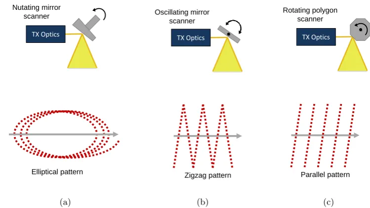
1.3 Examples of theoretical LiDAR scanning patterns: (a) elliptical pattern, (b) zigzag pattern, and (c) parallel pattern. The presented spatial arrangement of the pulse returns is the one expected in case of flat surface. . . 13

1.4 Basic components of the TLS system acquisition: (a) example of scan partitioning. For each scan, different angular steps should be considered to have the same point density in the whole acquisition, and (b) example of terrestrial LiDAR data acquisition. By increasing the distance of the scanner from the target, the point density decreases. . . . 15

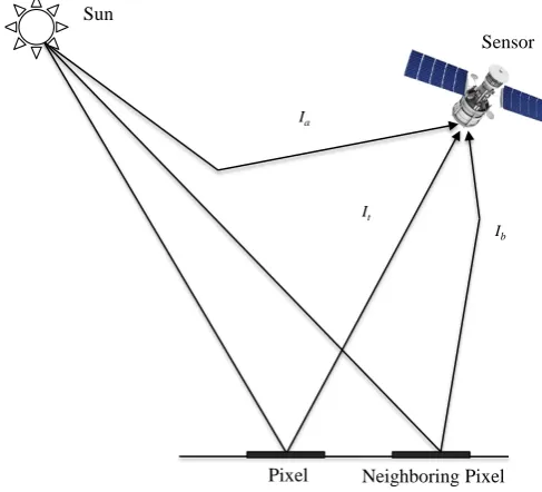
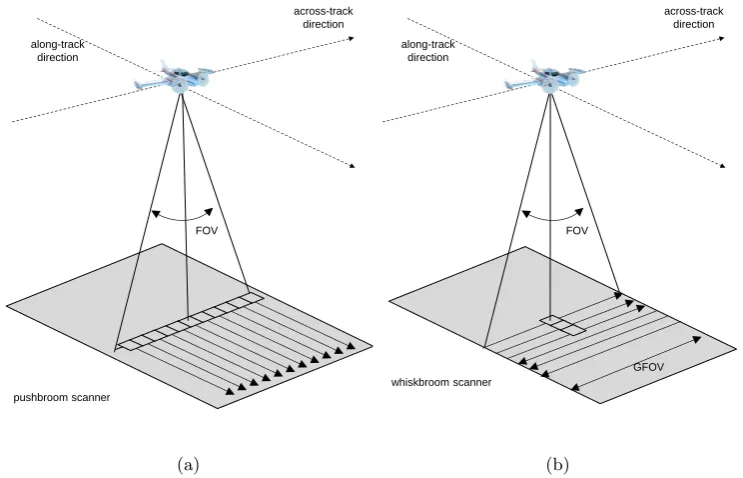
1.5 Representation of the main components that affect the radiance recorded by the sensor. 16 1.6 Examples of scanning methods for the acquisition of optical images: (a) pushbroom

scanner, (b) whiskbroom scanner. . . 17

2.1 Architecture of the proposed hierarchical approach to 3-D segmentation of the dominant and the sub-dominant crowns. . . 28

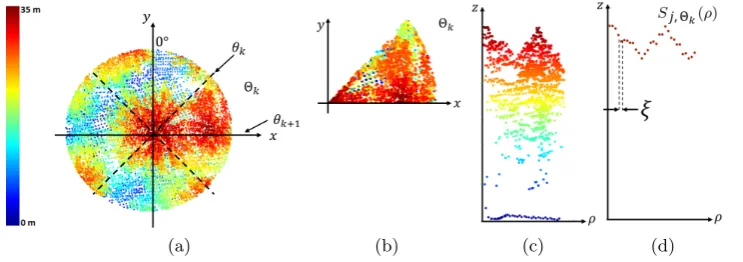
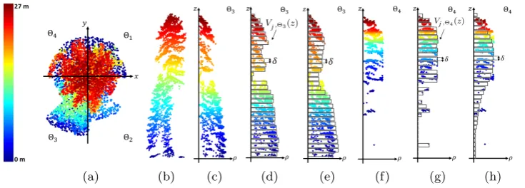
2.2 Example of angular analysis: (a) top view of the LiDAR point cloudPjdivided intoNθ

angular sectors, withNθ=8, (b) top view of the angular sector Θk, (c) side view of the

angular sector Θk after the circular projection, (d) side view of the 1-D discrete signal Sj,Θk(ρ) that approximates the shape of the crown in the sector Θk. . . 29

2.3 Example of sub-dominant tree crown detection: (a) top view of the dominant tree crown

Cjdivided intoLangular sectors, withL=4, (b) side view ofCj, (c) vertical profile of the

projected LiDAR points Πc(pi)∈Cj,Θ3, where the sub-dominant crown is present, (d)

vertical profile quantizationVj,Θ3(z), (e)Vj,Θ3(z) after the Gaussian filtering, (f) vertical

profile of the projected LiDAR points Πc(pi)∈Cj,Θ4, where no sub-dominant crowns

are present, (g) vertical profile quantization Vj,Θ4(z), (h) Vj,Θ4(z) after the Gaussian

filtering. . . 31

2.4 Example of sub-dominant tree detection: (a) top view of the dominant tree crown Cj

in the PCS, (b) top view of the sub-dominant tree in the PCS obtained keeping the set of LiDAR point Psub

j ={P sub j,Θ2,P

sub

j,Θ3}, (c) CHM of the dominant tree crown, and (d)

CHM of the sub-dominant tree crown, where the detected tree top is highlighted in red. 32

(18)

Plot H3, (d) Sample Plot H4, (e) Sample Plot H5, (f) Sample Plot H6, (g) Sample Plot H7. The rasterization has been performed with a spatial resolution of 25 cm. . . 34 2.6 False color representation of the CHMs representing the investigated stand plots for the

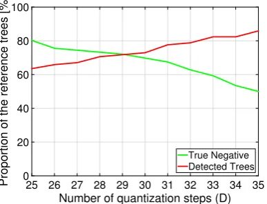
high-density LiDAR dataset. (a) Sample Plot M1, (b) Sample Plot M2, (c) Sample Plot M3, (d) Sample Plot M4, (e) Sample Plot M5, (f) Sample Plot M6. The rasterization has been performed with a spatial resolution of 50 cm. . . 34 2.7 Behaviour of the vertical quantization stepDvs the number of detected trees and true

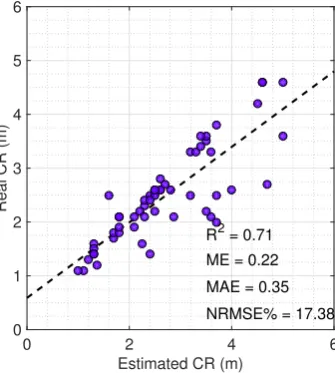
negatives for the sub-dominant layer of the forest. . . 36 2.8 Real versus estimated (with the proposed method) crown radius (CR) of the dominant

trees for: (a) the very high-density LiDAR dataset, (b) the high-density LiDAR dataset. 39 2.9 Qualitative example of tree crown segmentation obtained in the dominant layer of the

forest for: (a)-(f) the very high-density LiDAR data, and (g)-(l) the high-density LiDAR data. The segmented crowns (represented in bright colors) are located in the original forest scenario. A visual analysis confirms that the proposed method is able to properly extract trees both in dense canopy scenario and when they are isolated regardless of the laser point density. . . 40 2.10 Qualitative example of tree crown segmentation obtained in the sub-dominant layer

of the forest (very high-density LiDAR dataset). (a)-(f) the segmented crowns are represented in bright colors in the original forest scenario. . . 41 2.11 Real versus estimated (with the proposed method) crown radius (CR) of the

sub-dominant trees. . . 42

3.1 Architecture of the proposed method based on a data-driven identification of the tree growth models for an accurate DBH estimation. . . 45 3.2 Visual representation of the variables extracted to model the growth of the tree stems

in terms of: (a) the structure of the crown xTree_{, (b) the forest stand} _xPlot_{, (c) the}

topography xDtm_. _{. . . .} ₄₆ 3.3 Study area, Trentino region, Italy. The stand plots are highlighted in white and a zoom

of the two square stands points out the different forest density and structure conditions. 53 3.4 LiDAR tree heights vs DBH for: (a) all the considered trees, (b) the young trees classified

as ω1, (c) the mature trees classified as ω2, (d) the mature trees classified as ω3. For

each class, the DBH/height relationship is presented in black and overlapped on the scatterplots to highlight the different growth rates. . . 54 3.5 Features selected for the DBH estimation for: (a) the young trees ω1, (b) the mature

trees ω2, (c) the mature trees ω3. The features are represented in the ranking order

normalized between [0,1]. . . 56 3.6 Estimated vs real DBH obtained by using the multilinear regression model with (a) the

PM, (b) the RM. . . 57

4.1 Architecture of the proposed Tree Top Height Estimation Approach. . . 62 4.2 (a) RGB representation of the original ortophoto. (b) 3-D representation of the radiance

value of the green band. . . 64

(19)

4.3 (a) Representation of the tree crown parameters of the defined 3-D reconstruction model. (b) Example of 3-D model of the tree. . . 65 4.4 Example of classification based on the number of LiDAR points associated to the crown.

(a) LiDAR points shown in white and overlapped on the ortophoto, (b) both LiDAR pulses and crown boundaries represented in white overlapped on the ortophoto, and (c) crowns hit by more than one laser pulse (white), crowns hit by just one laser pulse (blue) and crowns missed by the laser scanner (red). . . 66 4.5 Example of the Tree Top reconstruction method for those crowns hit by just one LiDAR

point, withN = 3. For the generic tree, the 3 trees having similar point distances (d1,d2

and d3) and thus the 3 associated models (i.e., (cc1, ch1), (cc2, ch2) and (cc3, ch3)) are

tested. The chosen model is the one that returns the zt

j equal to the median value of

the 3 resultingzt

j. . . 68 4.6 Examples of the considered 3-D parametric model: (a) real scene, (b) LiDAR points

cloud of the trees, (c) 3-D parametric models of the trees automatically detected by the proposed method superimposed on the real scene, and (d) 3-D parametric models of the trees automatically detected by the proposed method superimposed on the LiDAR points cloud. . . 69 4.7 Optical images of the investigated area. (a) Stand plot P1, (b) Stand plot P2, (c) Stand

plot P1, (d) extended test area. . . 71 4.8 Masking procedure process. (a) Ortophoto of the Stand P2, (b) segmentation result

obtained on the ortophoto, (c) circular representation of the segmentation result, (d) masking process result using the lowest sampling density dataset (i.e., 0.25 pts/m2_),

(e) multisensor segmentation result, and (f) circular representation of the multisensor segmentation result. . . 73 4.9 Segmentation result obtained on the wide coniferous forest. The crown boundaries are

highlighted in white and overlapped on the ortophoto. . . 74 4.10 Reconstructed versus Observed Tree Top height for the trees hit by more than 1 LiDAR

point. The height estimation results of all the Stand Plots is presented for the dataset having density of: (a) 1 pt/m2_{, (b) 0.75 pts/m}2_{, (c) 0.5 pts/m}2_{, and (d) 0.25 pts/m}2_. _. ₇₅

5.1 The NEON Pacific Southwest domain (D17) is located in central California. It contains one core site and two relocatable sites. The core site, San Joaquin Experiment Range (SJER), is an oak savanna. . . 82 5.2 False color representation of the airborne CHM. The ideal TLS measurement setup is

in red and overlapped on the image, where for each position the acquisition number of the TLS scan is reported. Two example of TLS data are presented. . . 83 5.3 Block scheme of the proposed data fusion approach to the accurate reconstruction of

the 3-D structure of the crown. . . 84 5.4 Visual representation of the different LiDAR point sampling obtained by using ALS and

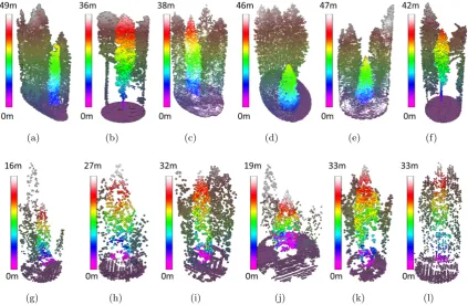
multi-angular TLS scans when considering the same tree. Due to the different view point, the LiDAR point cloud obtain are not comparable. . . 85 5.5 Example of point cloud fusion results. Due to the high resolution data obtained, the

three main species of the considered study area can be recognized by considering the different crown structures. . . 89

(20)

and superimposed on the nth terrestrial scan, (c),(f),(i),(l) crown boundaries of the registered airborne segmented imageSA

n

0

are superimposed on thenth terrestrial scan. . 92 5.7 TLS scan registration results: (a),(d),(g),(j) original terrestrial data, (b),(c),(h),(k)

crown boundaries of the original airborne segmented image SA _{are highlighted in gray}

and superimposed on the nth terrestrial scan, (c),(f),(i),(l) crown boundaries of the registered airborne segmented imageSA

n

0

are superimposed on thenth terrestrial scan. . 93 5.8 TLS scan registration results: (a),(d),(g),(j) original terrestrial data, (b),(c),(h),(k)

crown boundaries of the original airborne segmented image SA _{are highlighted in gray}

and superimposed on the nth terrestrial scan, (c),(f),(i),(l) crown boundaries of the registered airborne segmented imageS_nA0 are superimposed on thenth terrestrial scan. . 94 5.9 TLS scan registration results: (a),(d),(g),(j) original terrestrial data, (b),(c),(h),(k)

crown boundaries of the original airborne segmented image SA are highlighted in gray and superimposed on the nth terrestrial scan, (c),(f),(i),(l) crown boundaries of the registered airborne segmented imageSA

n

0

are superimposed on thenth terrestrial scan. . 95 5.10 TLS scan registration results: (a) original terrestrial data, (b) crown boundaries of the

original airborne segmented imageSA_{are highlighted in gray and superimposed on the} nth terrestrial scan, (c) crown boundaries of the registered airborne segmented imageSA

n

0

are superimposed on the nth terrestrial scan. . . 96

6.1 prova . . . 102 6.2 Example of hierarchical partitioning of the land-cover classes where the generic classck

is represented connected to its parent class M(ck) and its child-classesF(ck). In the considered examplefk is equal to three. . . 104 6.3 Color composition of the orthophoto acquired on a portion of the Trentino region. The

study areas are highlighted in the white rectangles overlapped on the optical image. A small portion of the high resolution optical images of the dataset is represented for both the study areas. . . 108 6.4 Hierarchical tree structure derived at the end of the invariance analysis for the considered

DA problem.. . . 110 6.5 Distributions of the labeled samples ofPad (left) andVds(right) represented in: (a-b)

the invariant feature subspace defined by the NDVI (hyperspectral scanner) and the height (LiDAR sensor), and (c-d) the feature subspace defined by the 16 and 37 spectral channels at the wavelength of 538 nm and 737 nm, respectively. . . 111

(21)

List of Abbreviations

AL Active Learning

ALS Airborne Laser Scanning

ALTM Airborne Laser Terrain Mapper

ALI Advanced Land Imager

BHC Binary Hierarchical Classifier

CCD Charge Coupled Device

CHM Canopy Height Model

COM Commission errors

CR Crown Radius

CRS Canopy Reflection Sum

DA Domain Adaptation

DBH Diameter at Breast Height

DET Detection accuracy

DGPS Differential Global Positioning System

DSM Digital Surface Model

DTM Digital Terrain Model

ECBD Enhanced Clustering Based Diversity

EO Earth Observing

ETM Enhanced Thematic Mapper

FOV Field Of View

FWHM Full Width at Half Maximum

GCC Global Canopy Cover

GFOV Ground Field Of View

GIFOV Instantaneous Ground Field of View

GLS Generalized Least Square

GWR Geographically Weighted Regression HFD Height Frequency Distribution IFOV Instantaneous Field of View INS Inertial Navigation System

ITC Individual Tree Crown

JM Jeffreys-Matusita distance

k-NN k Nearest Neighbor

LCC Local Canopy Cover

LCS Laser Cross Section

LiDAR Light Detection and Ranging

(22)

LMS Laser Measurement Systems

LSM Level Set Method

MAE Mean Absolute Error

MCLU Multi Class Level Uncertainty

ME Mean Error

MSE Mean Square Error

NDVI Normalized Difference Vegetation Index NEON National Ecological Observatory Network NRMSE Normalized Root Mean Square Error

OA Overall Accuracy

OAA One Against All

OLS Ordinary Least Square

OM Omission errors

P3_SVM _{Progressive Semisupervised Support Vector Machine}

PA Producer Accuracy

PCS Point Cloud Space

PDF Probability Density Function

PM Proposed Method

PRF Pulse Repetition Frequency R2 _{Coefficient of Determination}

RBF Radial Basis Function

RMSE Root Mean Square Error

RMSE(%) Percentage Root Mean Square Error

RS Remote Sensing

SFFS Sequential Forward Feature Selection SPOT Satellite Pour l’Observation de la Terre SSD Sum of Squared Differences

SSL Semi Supervised Learning

SVM Support Vector Machine

TCA Transfer Component Analysis

TLS Terrestrial Laser Scanning

TR Training

TS Test

UA User Accuracy

(23)

List of Symbol

Pt Transmitted power

Pe Received power

Rt Range between LiDAR and target

ϑBW Laser beam width

σ Laser cross section

A Aperture of the receiving lens

Oef f Optical efficiency of the TX-RX chain

Dl Lens Diameter

λ Laser wavelength

c Light speed

f Focal lenght

w Detector width

Ia radiance scattered by the atmosphere

It radiance reflected by the target and transmitted to the sensor

Ib radiance reflected by the background

P Normalized LiDAR point cloud (PCS)

TCHM Set of dominant tree-top detected in the CHM

p_i = (xi, yi, zi) Ground coordinates of the LiDAR point

tj = (xtj, ytj, zjt) Ground coordinates of the tree top

Pj Set of LiDAR points extracted around the tree top tj

Rs Search radius

Nθ Number of angular sectors used for the 3D crown segmentation

Θk Angular partition between the adjacent angles θk and θk+1 Pj,Θk LiDAR points belonging to the angular sector Θk

Sj,Θk(ρ) 1-D discrete signal representing Pj,Θk

Πc Circular projection that maps the points into the ρz plane

ξ Quantization step of the distance of the points from the tree-top

F Number of horizontal quantization steps

S_j,0_Θ

k(ρ) Discrete derivative of Sj,Θk(ρ)

Mj,Θk Closest height maximum to the tree-toptj of the angular sector Θk TPCS Set of dominant tree-top detected in the PCS

Tsub _{Set of sub-dominant tree top}

Ej,Θk Closest height minimum to the tree-toptj of the angular sector Θk C Set of dominant segmented tree crowns

(24)

Vj,Θk(z) 1-D vertical signal representing Πc(Cj,Θk), with pi = (zi, ρi) D Number of vertical quantization steps

δ Quantization step of the vertical profile of dominant tree

Hj,Θk Maximum height value of the set of points Cj,Θk H_j,sub_Θ

k Height of the sub-dominant tree detected in the angular sector Θk Psub

j,Θk Set of LiDAR points pi ∈ C sub

j,Θk havingzi ≤H sub j,Θk. Tsub _{Set of dominant tree-top detected in the CHM} Psub

k LiDAR point sectors associated to the sub-dominant tree-top Csub _{Set of sub-dominant segmented tree crowns}

xTree _{variables modeling the structure of the tree}

xPlot _{variables modeling the stand density}

xDtm _{variables modeling the topography}

z =g(x, y) DTM

gx = ∂z_∂x partial derivatives along x

gy = ∂z_∂y partial derivatives along y

gxx = ∂

2_z

∂x2 partial derivatives along xx gyy = ∂

2_z

∂y2 partial derivatives along yy gxy = ∂

2_z

∂x∂y partial derivatives along xy

p (g2

x+gy2)

q (g2_x+g_y2+ 1)

Hr

max Maximum height per return, with r=[1,4]

Hr

range Height range per return, with r=[1,4]

Hr

av Average height per return, with r =[1,4]

Hr

var Variance height per return, with r=[1,2]

Hr

skw Skewness height per return, with r=[1,2]

Hr

kurt Kurtosis height per return, with r=[1,4]

H1

max-H3max Max height 1st - Min height 3rd

H1

av - H2av Average height 1st - Average height 2nd

H1

av - H3av Average height 1st - Average height 3rd

H1

av - H4av Average height 1st - Average height 4th

H2

av - H3av Average height 2nd - Average height 3rd

H2_av - H4_av Average height 2nd - Average height 4th H3_av - H4_av Average height 3rd - Average height 4th

Hp pth height percentile, with p={25,50,75,90,95}

Ca Crown area

r1 Radius of the circle circumscribed to the crown r2 Radius of the ellipse circumscribed to the crown p2/p1 Ratio of 2nd and 1st return pulses (in a radius = 10m)

Swest Slope between (xt, yt) and (xt−10 m , yt)

Seast Slope between (xt, yt) and (xt+ 10 m, yt)

Ssouth Slope between (xt, yt) and (xt, yt−10 m)

(25)

Snord Slope between (xt, yt) and (xt, yt+ 10 m)

γ Aspect (degrees clockwise from north)

ϕ Profile Curvature: direction of max slope

φ Plan Curvature: transverse to the max slope

w Wetness Index

Amin Minimum Altitude

Amax Maximum Altitude

Aav Average Altitude

ΩM ={ωi}Mi=1 M growth model classes

xEnv _{Environmental feature space} {υi} cluster center

Bht Bhattacharyya distance of the classes ωh and ωt

J Mht JM distance of the classes ωh and ωt

µh Mean vector of class ωh,

Σh Covariance matrix of class ωh

y_i vector of observed DBH values Xi matrix of extracted variables

βi vector of model parameter estimation

εi residual error

Q Structural element chosen for dilating the CHM image

DCHM Domain of the image CHM

DQ Domain of the structuring element Q

thHeight Height threshold

Msk Mask Image

G Green band of the optical image

Gm Masked green band of the optical image

N Number of LiDAR pulses associated to each crown

nj Number of LiDAR pulses associated to the crown Cj

ch Crown height

cc Crown curvature

cr Crown radius

ri(¯zjt) Residual of the ith LiDAR point

dref distance of the LiDAR point from the center of the tree

Nm Possible tree models

PT

n Normalized nth terrestrial LiDAR scan PA _{Normalized airborne LiDAR data}

ζn Geometric affine transformation

IA _{CHM of the airborne LiDAR data}

I_nT CHM of the nth terrestrial LiDAR scan

SA segmented image

CA _{Set of airborne segmented crown}

I_nA Portion of the airborne image having the same size of I_nT

φ Rotation angle

[sx, sy] Scaling factor

(26)

Υ Correlation coefficient

µT

n Mean value of InT

µA_n Mean value of I_nA0

CT

n Set of segmented LiDAR point clouds of InT

Ψn nth sensor

xΨn _{Feature vector extracted by the} _n_{th sensor}

Ω ={ωm}M

m=1 M land-cover classes DS ={XS,YS} Source domain DT ={XT} Target domain

P(ωm) Prior probability of ωm

p(x|ωm) Class conditional probability of ωm

pS_(x) _{Distribution of the source domain}

pT_(x) _{Distribution of the target domain}

Call Set of classes of the hierarchical tree structure

M(ck) Parent class of ck

F(ck) Set of child classes

Cv ⊆ Call Subset of classes for which none of the sensors available can measure

invariant features

Cinv ⊆ Call Subset of classes for which at least one sensor available is able to measure spatial invariant features

XT

ck Unlabeled samples of the target domain belonging to ck TS

ck Training set of DS for the considered invariant classes ck

w Vector normal to the separating hyperplane

b Bias term

C Regularization parameter

ξ_is Slack variable associated with thensck labeled samples of the source

domain for the classes ck1 and ck2 αs_i Lagrange multipliers, with i= 1, .., nsck

xs i ·xsj

Inner product between the two feature vectors xs

i and xsj

Φ(x) Nonlinear mapping function to project the samples into an higher dimensional space

K(xs

i,xsj) Kernel function

G Subset of training samples corresponding to the nonzeros Lagrange multipliers

XT

ck Target unlabeled samples

f(x) SVM hyperplane

TT

ck(0) Initial training set of DT TT

ck(1) Training set including all the original unlabeled samples X T ck TT

inf Initial training set for all the Cinv classes of DT

(27)

Introduction

This chapter presents an introduction to the PhD thesis work. We briefly introduce the framework where this work has been developed by providing an overview of the problem of forest parameter estimation using remote sensing data. This allows us to highlight and discuss the motivation, the objectives and the novel contributions of this thesis. Finally, the structure of the document is reported.

Background

Nowadays, the accurate estimation of forest parameters at individual tree level has become an important research topic. Precision forestry is the new direction of modern forest inventories, which aims to obtain a comprehensive representation of the tree structure for better forest management. In this framework, the integration of different remote sensing sources represents an effective solution to obtain precise analysis of the forest parameters. This calls for the development of novel methods being able to exploit the complementary information provided by the different data sources. Moreover, the new generation of high resolution sensors results in the collection of an overwhelming amount of detail of the forest. The availability of this large amount of information encourages the definition of automatic techniques being able to exploit the full potential of these data for an accurate estimation of the forest parameters. In the following a brief overview on the use of remote sensing data for forest parameter estimation is given.

Remote sensing data have been widely employed to estimate forest parameters due to the possibility of monitoring objectively and accurately large forest areas. The traditional approach, based on field observations, is constrained by lack of access to remote areas (especially in mountainous scenarios) and involves high costs related to the amount of time spent for collecting field data. Moreover, in order to obtain reliable estimates, the number of ground measurements collected should be proportional to the extension of the considered forest area. Therefore, this approach is efficient when applied to small areas, but at regional scale the data collected could be not sufficient for modelling accurately the entire investigated area. In this framework, remote sensing represents a valuable technology for providing measures useful for forestry inventories. In particular, in this thesis we focus the attention on Active Light Detection and Ranging (LiDAR) sensor and passive high spatial/spectral resolution optical sensors.

(28)

the tree crowns and allows the 3-D reconstruction of the forest. The acquisition of LiDAR data can be carried out by either Airborne Laser Scanning (ALS) systems or Terrestrial Laser Scanning (TLS). ALS systems are suited for surveying and mapping large forest areas, whereas TLS data are usually employed for local forest inventories. When acquired with high laser sampling density (i.e., characterized by a number of hits per m2 _higher

(29)

Introduction 3

In this framework, the integration of these data sources represents an effective solution to obtain precise analysis of the forest parameters. However, in order to cope with this large amount of data, it is necessary to develop techniques that can automatically achieve accurate forest parameters estimations by fusing the information provided by different data sources.

Another important research topic in forestry is related to the precise land cover map-ping of the forest area and the forest species. To obtain reliable classification maps, supervised classification methods are usually employed. The main drawback of these methods is the need of a sufficient number of labeled ground reference samples for train-ing the classification algorithm. However, in many cases reference samples are expensive and difficult to collect. Therefore, in real application scenarios, it is not reasonable to as-sume to have groundtruth available on wide forest area. To mitigate the need of labeled samples, the classification of a remote sensing data where no ground data is available (target domain) can be performed by using ground reference data associated to a data acquired by the same sensor in a region with comparable properties (i.e., the same set of land-cover classes). However, even tough the data are similar to each other, it is necessary to face many problems. The different acquisition conditions of the two data (e.g., illu-mination conditions, atmosphere conditions, look/view angles, sensor parameters) affect the radiometry of the scene. Moreover, the phenological state of the vegetation or the differences in the soil moisture can lead to crucial variations in the spectral response of the same land-cover classes. In machine learning and pattern recognition literature, these problems are usually addressed by domain adaptation (DA) methods. The main idea is to model the changes between similar domains by transferring the knowledge learned on the source domain (one or more) to a target domain. DA methods address critical and challenging problems due to the fact that labeled data are assumed to be available only for the source domain, which is different from the target domain. It is clear that in such a complex scenario the accuracy of the obtained results is strongly related to the capability of modelling properly the changes occurring between the two image domains. In this framework, the availability of multiple remote sensing data sources results in the collection of complementary measurements of the classes. By exploiting the capability of each sensor of measuring different physical properties of the scene it is possible to increase the reliability of the obtained results.

Objectives and Novel Contributions of the Thesis

The work presented in this thesis is aimed at investigating and defining novel methods for the precise estimation of forest parameters by exploiting the properties of different remote sensing data sources. In particular, we focused the attention on the main gaps present in the literature towards the direction of the precision forestry. Accordingly, it is necessary to develop automatic methods capable of exploiting the full potential of the new generation of high resolution LiDAR sensors and to define data fusion techniques being able to accurately integrating the different information provided by multiple remote sensing sources. In greater detail, the novel contribution of the thesis are as follows:

(30)

high-density LiDAR data.

2. An adaptive tree stem diameter estimation technique for high-density LiDAR data.

3. A tree top height estimation method based on the fusion low-density LiDAR data and high resolution optical images.

4. A crown structure estimation method based on the fusion of airborne and terrestrial LiDAR data.

5. A sensor-driven DA method for the classification of large forest areas with multisen-sor data.

In the following subsections the main objectives and novelties per contribution of the thesis will be briefly described.

Hierarchical 3-D Crown Segmentation Method

As mentioned above, the accurate estimation of forest parameters at individual tree level is becoming essential for modern forest inventories. The estimation of the tree parameters requires the segmentation of the single tree crowns including the dominant trees and the understory vegetation. Thus, in this thesis we present a novel method for the detection and delineation of the single tree crowns in multilayered forest by using very high-density LiDAR data. The proposed method performs a 3-D segmentation of both the dominant and the sub-dominant trees visible in the LiDAR point cloud. Unlike the methods present in the literature, the proposed approach does not require any prior knowledge on the crown size and forest density, but relies on the geometrical structure of the forest and the properties of the LiDAR data. Thus, it can be successfully applied to large forest areas characterized by heterogeneous 3-D crown structures. The method considers both the rasterized version of the LiDAR data (i.e., image domain) and the original point cloud domain. The main novelties of the proposed approach are: (i) the use of the LiDAR point cloud to detect the dominant trees missed in the image domain, (ii) the identification of the sub-dominant trees located in different sides of the dominant tree crowns by means of an angular analysis, and (iii) a crown delineation method for both dominant and sub-dominant trees based on the derivative analysis of the horizontal profile of the trees in the LiDAR point cloud. The effectiveness of the proposed method is demonstrated in experiments carried out in a complex dense forest scenario located in the Southern Alps of the Trentino region (Italy) by using very high-density LiDAR data (up to 50 pts/m2) and high-density LiDAR data (up to 5 pts/m2_).

Adaptive Tree Stem Diameter Estimation Method

(31)

Introduction 5

DBH are usually overestimated and underestimated, respectively. These errors lead to a wrong reconstruction of the forest structure as well as a wrong estimation of the forest volume. To solve this problem, we propose an adaptive method to the accurate estima-tion of the DBH. First, the main tree growth model classes are detected by means of a data-driven approach. Then, for each growth model class, a tailored regression rule is defined and used to improve the estimation accuracy of small and large stem diameters. All the factors which can affect the growth of the tree stem in terms of topography and forest density are modeled. Differently from the literature, the proposed approach: (i) performs a data-driven detection of the growth model classes, (ii) allows an accurate rep-resentation of the environmental factors which affect the DBH growth, and (iii) defines different regression models for each growth model class. Experiments were carried out on high-density LiDAR data in a forest area characterized by a wide range of stem diameters. The results show that the method has a high estimation accuracy regardless of the size of the tree stem.

Tree Top Height Estimation Method

One of the most important forest parameter that needs to be accurately estimated is the height of the trees. Due to the high acquisition costs of high-density LiDAR data, when dealing with large forest areas low-density data are typically acquired. However, the reduction of the number of laser points results in: (i) an underestimation of the height of the trees, (ii) the missed detection of some trees present in the scene. To mitigate the lack information due to the low laser sampling, thus improving the estimation results, low cost high resolution optical images can be employed. Accordingly, by integrating the accurate representation of the horizontal structure of the forest provided by the optical data to the vertical height information of the LiDAR sensor, we aim to reconstruct the tree top height by means of a 3-D tree model representing the crown structure. Moreover, the heights of the missed trees are estimated by means of a k-Near Neighbours trees (k-NN trees) technique which takes advantage from the correlation between tree height and crown area. The main novelties of the proposed technique are: (i) the use of a 3-D parametric model for the reconstruction of the tree top height of those crowns hit by LiDAR points, and (ii) the estimation of the tree top height for those crowns that are missed by any LiDAR pulse with a k-NN trees technique. In this study, we concentrate our attention on coniferous forests in the Alpine scenario. In the experiments, we considered four LiDAR datasets of low laser sampling density (i.e., 1, 0.75, 0.5, and 0.25 pt/m2_{) and very high resolution}

optical images (0.20 m). The experimental results obtained confirm the effectiveness of the proposed technique.

A Method for Crown Structure Estimation based on the Fusion of Airborne and Terrestrial LiDAR data

(32)

we present a method that integrates the terrestrial and low-density airborne LiDAR data for the accurate crown structure estimation for localized forest analysis. TLS data are typically acquired to replace traditional forest inventories, thus used as reference data to estimate forest parameters using ALS. However, despite the increasing availability of the two data types on the same forest area, few papers address the fusion of these data source. Moreover, to the best of our knowledge, the fusion of these data is usually performed considering the synthesis of derived parameters rather than integration of the ALS/TLS data from a real fusion view point. Based on this knowledge gap, we propose an automatic data fusion technique that aims to exploit the complementarity of these data to accurately estimate the 3-D structure of the forest stand and model the structure of the crowns. The main novel contributions of this method are: (i) the use of the ALS data for the automatic registration of the multiple terrestrial scans (without the need for reference targets), (ii) the analysis of the forest spatial pattern to perform the registration of the data, (iii) the use of the airborne segmentation results to delineate the crown in the TLS scans, and (iv) the integration of the 3-D LiDAR point clouds. The experimental results obtained in an open woodland forest scenario demonstrate the importance of fusing the two LiDAR point clouds to accurately represent the crown structure.

Classification of Large Forest Areas by a Sensor-Driven Domain Adaptation Method

(33)

Introduction 7

Thesis Organization

The present Chapter provided a brief overview on the use of remote sensing data for forestry application. In addition, it introduced the motivation, the objectives and the novel contributions of this thesis. The rest of this dissertation is organized in six main chapters. Chapter 1 illustrates the fundamentals and the background notions useful for understanding the thesis. Moreover, a brief analysis of the state-of-the-art on the use of remote sensing data for forest parameter estimation is presented. Chapter 2 introduces to the main problems related to the single tree crown segmentation in multilayered forest by using LiDAR data. Then, it presents the proposed novel 3-D segmentation approach to the detection and the delineation of dominant crowns and understory vegetation, which takes advantage from the properties of the very high resolution LiDAR sensor. Chapter 3 proposes an adaptive data-driven method based on the detection of growth model classes for an accurate estimation of the DBH by using high-density LiDAR data.

In the framework of the fusion of multisensor remote sensing data, Chapter 4 illustrates the proposed 3-D model based approach to the accurate tree top height estimation, which is based on the fusion of low-density LiDAR data and high resolution optical images. Chapter 5 presents the fusion of low-density airborne and terrestrial LiDAR data for an accurate 3-D canopy structure characterization, whereas Chapter 6 reports the novel sensor-driven DA method for transferring the knowledge between remote sensing data acquired on different forest areas but sharing similar properties.

(34)

(35)

Chapter 1

Fundamental and Background

In this chapter we review the fundamentals of remote sensing data used in this thesis. In the first section we provide the concepts and definitions needed throughout the disserta-tion. In particular, we illustrate the basic principles of LiDAR sensor mounted on both airborne and terrestrial platforms, and passive high spatial/spectral resolution optical sen-sors. Then, a brief analysis of the state-of-the-art regarding the use of remote sensing data for forest parameter estimation is reported.

1.1

Fundamentals

In the framework of remote sensing technologies, two main classes of sensors can be dis-tinguished: active sensors and passive sensors. Active sensors generate and direct energy toward a target and subsequently record the backscattered radiation. Most common ac-tive sensors are RADAR (radio detection and ranging) and LiDAR (light detection and ranging). In this thesis we focus the attention on LiDAR systems, which emit pulses of light by laser beams. This characteristic allows the acquisition of LiDAR data during the night, when the air is usually clearer. However, unlike RADAR systems LiDAR sensors cannot penetrate clouds, rain, or dense haze due to the working wavelengths. Passive sensors measure the electromagnetic energy radiated and reflected by the Earth surface. The radiation measured by the passive systems comes from an emitting external source of energy (typically the sun in the visible and infrared portions of the spectrum), which propagates through the atmosphere and hits the Earth’s surface. The Earth’s surface in-teracts with the incident electromagnetic wave by absorbing, transmitting and reflecting the incident energy of the transmitted component. The reflected components propagate back through the atmosphere (again with absorption), thus reaching the sensor. In this thesis, we focus on the analysis of high geometrical and high spectral resolution optical images. In the following, the basic principle of LiDAR and passive optical sensors are presented.

1.1.1 LiDAR basis

(36)

the properties of the laser light reflected by the target. The sensor transmits a short-duration pulse of laser light towards the target, while the receiver (placed in the same location of the sensor) measures the elapsed time between emission and detection of the reflected light back at the sensor (Fig. 1.1). By using the speed of light, the time measure is then converted into the distance of the point from which the light was reflected. Similar to RADAR systems, but working at smaller wavelengths, LiDAR is highly sensitive to small targets such as aerosols and cloud particles and thus, it has also been used for atmospheric research. Most of the LiDAR systems operate in the near-infrared part of the electromagnetic spectrum (i.e., for forestry application typically between 1010 [nm] - 1064 [nm]), even though some sensors work in the green band to penetrate water and detect bathymetry features. Moreover, due to their very narrow beam, LiDAR data are characterized by a high geometrical resolution.

Let us focus the attention on the LiDAR transmission equation. The echo power Pe

received is a function of the transmitted powerPtand depends on four main contributions.

By assuming the laser beam larger than the target size and the source of power as a point isotropic radiator, the first contribution is the power density emitted by the source located at distance Rt over a spherical area, i.e.,:

Pt

(4π) R2 t

(1.1)

Accordingly, the echo power is affected by the return power density scattered over the forward hemisphere, i.e.,:

1 2π R2

t

(1.2)

The third factor that affects the power returned from the target is the directivity of the lens used to radiate the power in a given direction, which depends on the laser beam width ϑBW as follows:

4π π/4ϑ2

BW

(1.3)

Finally, the last contribution is given by the Laser Cross Section (LCS) σ, the aperture of the receiving lens A and the optical efficiency of the TX-RX chain Oef f. The LCS

estimates how detectable the object is for the laser pulse, and depends on the size and the chemical composition of the target and the wavelength. Accordingly, the relation of the transmitted laser power Ptto the echo power of its reflections Pe is given by the following

LiDAR transmission equation:

Pe=

Pt

4πR2 t

· 1

2π R2 t

· 4π

(π/4)ϑ2 BW

·σ·A·Oef f (1.4)

The laser beamϑBW depends on the lens diameterDland theλwavelength of the adopted

light radiation, i.e.,:

ϑBW =

λ Dl

=λ· r

π

(37)

Fundamentals 11

Laser

2 )

( p

t c t t

R  





Target Surface

Reflected pulse Trasmitted pulse

p

t t

t R

Figure 1.1: Basic principle of LiDAR sensor.

Thus, the LiDAR transmission equation can be rewritten as follows:

Pe =

8A2·Pt·σ·Oef f

π3_R4 tλ2

(1.6)

In Fig. 1.1 the basic principle of the sensor is illustrated. The target surface placed at distanceRtis hit by the pulse emitted at timetp. At timetthe energy is observed back at

the laser location. The distance of the target from the scanner is estimated according to the speed of light and time difference between the pulses, which is halved due to the round-trip. In real application scenario, when the laser emit the light pulse, the sensor position in terms of latitude, longitude and altitude are recorded in order to convert the position of the target in geographic coordinates (x,y,z). At the end of the acquisition phase, the outcome of the sensor is a 3-D point cloud, derived by the laser range measurements and the knowledge on the position and altitude of the instrument.

(38)

Flying altitude (2000 m)

Beam divergence

Footprint diameter

0.3 mrad 0.6 mrad

1.2 m 0.6 m

(a)

Scan angle

Scanning swath Scanning

line

Nominal footprint spacing between scanning lines Footprint spacing

along scanning lines

Roll Pitch

Heading

(b)

Figure 1.2: Principle of ALS system: (a) example of LiDAR beam divergence, for a given flying altitude the footprint diameter depends on the laser beam of the sensor, (b) representation of the main scanning attributes of airborne LiDAR data acquisition considering a zizag scanning pattern.

they result in an accurate representation of the 3-D shape and the inner structure of the target [2, 3].

The acquisition of LiDAR data can be performed by using different platforms according to the application. In this thesis we focus the attention on the ALS and the TLS for forestry applications. In the following sections the two systems are described in detail.

1.1.2 Airborne Laser Scanning (ALS)

ALS systems consist of a set of instruments that work independently: (i) the laser device, (ii) a Differential Global Positioning System (DGPS) which records the geographic po-sition for each collected point, (iii) an Inertial Navigation System (INS) which monitors the flight dynamic by recording the parameters related to the rotation angles of the vehi-cle (pitch, roll and yaw) and the horizontal and vertical movements of the aircraft (Fig. 1.2b), and iv) a computer interface that manages communication among devices and data storage.

(39)

Fundamentals 13

Elliptical pattern

TX Optics

Nutating mirror scanner

(a)

TX Optics

Oscillating mirror scanner

Zigzag pattern

(b)

TX Optics

Rotating polygon scanner

Parallel pattern

(c)

Figure 1.3: Examples of theoretical LiDAR scanning patterns: (a) elliptical pattern, (b) zigzag pattern, and (c) parallel pattern. The presented spatial arrangement of the pulse returns is the one expected in case of flat surface.

diameter depends on the beam divergence and the flying altitude. In greater detail, it is defined as the beam diameter intercepted by a plane positioned perpendicularly to the beam direction at a distance from the instrument equal to the nominal flying altitude. Fig. 1.2a presents a practical example where, for the same flying altitude (i.e., 2000 m), different footprint diameters are obtained because of the different beam divergence. Indeed, even though in a true laser system the trajectories of the photons generate a cylinder, in a beam emitted by a LiDAR instrument their trajectories slightly deviate, thus forming a narrow cone. By increasing the distance between the laser and the target, the footprint diameter increases. To obtain an accurate representation of the forest structure, small footprint (i.e., 0.1m - 2 m) are preferred because they facilitate accurate linkages between the LiDAR point cloud and the individual trees or forest stands. Indeed, the distribution of the pulse energy is not uniform within the footprint, thus it is usually approximated with 2-D Gaussian distributions since it radially decreases from the center.

(40)

(50 kHz and 100 kHz), different forest parameter estimation are obtained, especially for metrics derived from the last echoes. The scan angle is defined as the off-nadir angle at which the sensor acquires during scanning. By increasing the scan angle it is possible to reduce the acquisitions cost, because of the possibility of covering more ground in a single flight line. However, canopy penetration deteriorates at higher values of scan angles. Moreover, height measurement errors are visible with scan angles >10◦ off-nadir [5].

To collect the LiDAR point cloud all over the considered scene, the direction of the laser beam needs to be moved across the flight direction while the aircraft is moving since it can illuminate a single point at once. Depending on the mechanism used to direct pulses across the flight lines, multiple types of patterns are defined. Indeed, during the ALS acquisition, the laser beam is pulsed towards a mirror and projected downward from the aircraft. Moreover, the beam is scanned from side to side by a moving optics as the aircraft flies over the investigated area according to a specific scanning pattern. Fig. 1.3 presents the most common scanning patterns employed. Even though the configuration is usually designed to preserve equal spacing between returns, in real acquisition scenarios pulse density is not uniform and laser density eventually is higher at the end of the swath because of mirror deceleration. However, according to the scanning pattern, the footprint spacing along the scanning lines and the nominal footprint spacing between the scanning lines can be calculated (Fig. 1.2b).

1.1.3 Terrestrial Laser Scanning (TLS)

TLS systems refer to LiDAR acquisition performed from a static view point, typically a tripod, thus creating a 3-D point cloud of the surrounding vegetation. In the framework of forest parameter estimation, TLS is typically acquired for accurate local forest invento-ries. Indeed, it is a valuable tool for retrieving tree parameters because of its capability of recording high resolution profiles of the individual tree crowns. Moreover, the 3-D point cloud provided by the laser scanner solves the limitations in structural detail which can be measured by conventional forest inventory. Similarly to the airborne sensor, the basic concept of this system is the use of light to determine the target distance. TLS systems were initially developed for engineering and mining applications, with characteristics (e.g., cost, resolution, acquisition efficiency, portability) that precluded a favorable cost-benefit for forestry applications. However, in recent years the development of portable and cost-effective TLS increased the possibility of performing efficient forest structure assessment using these systems. The survey equipment used to collect TLS data include tripods, tar-gets, tribrachs, target poles, and a laptop computer. Typically the radial survey method is used for the terrestrial data acquisition. The basic components of the TLS system are shown in Fig. 1.4.

(41)

Fundamentals 15 (a) Φ" θ" x" y" z" r" d1 d2 Φ" θ" x" y" z" r" Φ" θ" x" y" z" r" Φ" θ" x" y" z" r" Φ" θ" x" y" z" r" (b)

Figure 1.4: Basic components of the TLS system acquisition: (a) example of scan partitioning. For each scan, different angular steps should be considered to have the same point density in the whole acquisition, and (b) example of terrestrial LiDAR data acquisition. By increasing the distance of the scanner from the target, the point density decreases.

recorded by the receiver. Thus, the wider is the illuminated area, the less overall detail is gained on a scale smaller than the illuminated area. Together with the beam divergence, the resolution of the terrestrial LiDAR data is affected by the angular resolution, which influences the point density. The point density of the TLS systems depends on the distance of the target and the angular step. The higher is the distance of the target from the scanner, the lower is the point density acquired (Fig. 1.4b). However, by decreasing the angular step of the laser beam, the spot space decreases, improving the spatial resolution of the data. Thus, to obtain a high resolution scan at long ranges, the angular step should be tuned considering the distance from the target. In particular, this parameter can be adjusted in the vertical and the horizontal directions in order to obtain a very high points density acquisition. It is worth noting that extremely dense point clouds require more storage space and take a longer time to scan. This impacts both the time spent out in the field collecting data and the data processing computational complexity. Finally, the terrestrial LiDAR acquisitions are strongly affected by the topography of the scene because of the varying ranges of the objects measured by the sensor within the same scan. For this reason, in order to obtain a homogeneous point density acquisition in the entire scene, the scan needs to be partitioned into several scans at determined mean distance intervals (Fig. 1.4a). Then, the angular step should be adjusted as a function of that mean distance to achieve the same resolution and point density. In particular, since TLS scans along vertical and horizontal orientations, vertical and horizontal partitioning needs to be taken into consideration during a complex project.

1.1.4 Passive Optical Sensors

(42)

Ia

I_t

Ib

Pixel Neighboring Pixel

Sensor Sun

Figure 1.5: Representation of the main components that affect the radiance recorded by the sensor.

without the sun radiation. The solar radiation spectrum can be modeled by a black body with source temperature of 5900 K, with a peak radiation located at wavelength of about 500 nm. The signal measured by the sensor is mainly the radiation coming from the sun, which is reflected by the Earth’s surface passing through the atmosphere. A small amount of energy is also directly emitted by the Earth’s surface. The interaction between the solar radiation and the gas molecules present in the atmosphere strongly affects the solar radiation. Thus, only the wavelength regions of the electromagnetic spectrum where the atmospheric gas absorption effect is minimized can be used for remote sensing. Fig. 1.5 shows a schematic representation of the main components that affect the radiance recorded by the sensor which are: (i) the radiation scattered by the atmosphere Ia in

the viewing direction, (ii) the radiance reflected by the target It and transmitted to the

sensor, and (iii) the radiation reflected by the background Ib. The measured radiance

hit the electronics detectors (i.e., the Charge Coupled Device (CCD)) placed on the focal plane. The signal focused by the optics of the imaging system is converted into electrical current to obtain the digital image and be stored.

In a real acquisition scenario, the energy emitted by a point source is spread over the finite size of the cells of the CCD sensor. This effect, due to the sensor’s focal length f

(43)

Fundamentals 17

FOV along-track

direction

across-track direction

pushbroom scanner

(a)

FOV along-track

direction

across-track direction

GFOV whiskbroom scanner

(b)

Figure 1.6: Examples of scanning methods for the acquisition of optical images: (a) pushbroom scanner, (b) whiskbroom scanner.

geometrical resolution of the optical image (i.e., pixel size). Thus, each pixel represents a portion of the investigated area enclosed in the angular cone of visibility of the sensor at a given flight altitude.

To generate the optical image, the scanning in the across-track direction (orthogonal to the motion of the sensor platform) is combined with the motion of the platform in the along-track direction. According to the number of detectors used to scan, different scanning patterns are used. Fig. 1.6 shows the main types of scanning patterns for the acquisition of optical images: the whiskbroom scanner and the pushbroom scanner. The whiskbroom scanner uses several CCD detectors aligned in track to achieve parallel scanning, thus acquiring more pixels simultaneously. However, to scan the entire scene a rotating mirror which moves back and forth across the flight direction is required. The mechanical rotating mirror limits the acquired spatial resolution due to slower data rates. The pushbroom scanner, also referred to asacross-track scanners, is a wide-angle optical system which uses a linear array of thousand of CCD detectors arranged perpendicular to the flight direction. While the aircraft flies forward, the scanner is acquiring one line at a time of the optical image. Although the detectors need to be perfectly calibrated to avoid striping artefacts, these systems allow the fast acquisition of high data rates. Thus, this technique is suited for high resolution sensors.

(44)

analyzed scene. For this reason, high spatial optical images represent an important source of information for environmental monitoring. However, the energy emitted by the source is quantized both from the spatial and the spectral view point. Thus, together with the spatial resolution, one of the most important characteristic of the optical sensor is the spectral resolution, which describes the sensitivity of a sensor to the wavelength interval. The finer is the spectral resolution, the narrower is the wavelength range for a partic-ular channel or band. To characterize the target, it is possible to analyze its reflecting behaviour at different wavelengths, i.e., its spectral signature. Indeed, depending on the chemical and physical characteristic of the object, the solar radiation can be transmitted, absorbed or reflected by the target surface in a different way in different portions of the electromagnetic spectrum. If the optical remote sensing system has a sufficient spectral resolution, the object can be identified by its spectral signature. Depending on the ap-plication, the main passive optical remote sensing sensors that can be considered are: multispectral sensors and hyperspectral sensors. Multispectral sensors are characterized by a few broad bands (< 10), whereas hyperspectral sensors have up to a few hundred of very narrow spectral bands. These data are a rich source of information for precise recognition and characterization of the material and objects on the ground, thus facilitat-ing fine discrimination between different targets based on their spectral response in each of the narrow bands. Hyperspectral images allow the precise identification of land-cover classes and thus, they are suited for application such as detailed classification of forest areas. In this thesis high spatial resolution and high spectral resolution optical images are considered.

1.2

Related Works: Remote Sensing and Forestry

The estimation of forest attributes has been effectively improved by the use of the remote sensing technology. The traditional approach to forest inventories is based on ground measurements that are collected for some stand plots usually chosen by randomly sampling a forest area. Then, these measurements are statistically extended to the entire area in order to obtain global estimates of the forest parameters (e.g., average tree volume, average tree height, tree density). For obtaining reliable estimates, the amount of data collected should be representative of the entire forest ecosystem considered. However, field surveys are costly, time consuming and constrained by lack of access to remote areas (especially in mountainous scenarios). In this context, remote sensing represents an important tool for monitoring objectively and accurately large forest areas. In the following a brief analysis of the state-of-the-art on the use of remote sensing data for forest parameter estimation is presented. In particular, in this thesis we focus the attention on LiDAR data and optical images even though SAR data have been employed for single tree detection [6, 7]. More details on specific topics will be given in the next Chapters.

1.2.1 Forest Parameters Estimation with LiDAR Data

(45)

Related Works: Remote Sensin