Published online March 4, 2015 (http://www.sciencepublishinggroup.com/j/ijber) doi: 10.11648/j.ijber.20150402.14
ISSN: 2328-7543 (Print); ISSN: 2328-756X (Online)
Determinants of Uganda’s Export Performance: A Gravity
Model Analysis
Henry Tumwebaze Karamuriro
1, Wilfred Nahamya Karukuza
21
Department of Economics and Statistics, Kyambogo University, Kampala, Uganda 2
Uganda Business and Technical Examinations Board, Kampala, Uganda
Email address:
[email protected] (H. T. Karamuriro), [email protected] (W. N. Karukuza)
To cite this article:
Henry Tumwebaze Karamuriro, Wilfred Nahamya Karukuza. Determinants of Uganda’s Export Performance: A Gravity Model Analysis. International Journal of Business and Economics Research. Vol. 4, No. 2, 2015, pp. 45-54. doi: 10.11648/j.ijber.20150402.14
Abstract:
Exports play an important role in Uganda’s economy, influencing the level of economic growth, employment and the Balance of Payments. Uganda has initiated several trade policy reforms aimed at promoting the export sector. However, Uganda’s share in total world exports is still very low. Given the central role of exports in the economy, it was important to identify the plausible factors affecting export flows between Uganda and its trading partners. Thus, this paper examines the factors affecting Uganda’s exports using an augmented gravity model of trade. The panel dataset used was for the period 1980 to 2012. The results suggest that Uganda’s GDP, importer’s GDP, importer’s GDP per capita, per capita GDP difference between Uganda and its trading partners, real exchange rate, official common language, and contiguity had a positive and statistically significant effect on Uganda’s exports. The study further, shows that the formation of COMESA and EAC had a significant positive effect on Uganda’s exports. On the other hand, Uganda’s GDP per capita and distance between Uganda and its trading partners had a negative effect on Uganda’s export flows. These results are important for trade policy formulation in order to ensure that Uganda’s export potential is exploited so as to enhance economic growth.Keywords:
Gravity Model, Fixed Effects Regression, Random Effects Regression, Instrumental Variables GMM Regression,Exports
1. Introduction
The failure of the in-ward looking policies to stimulate the desired growth in Sub-Saharan Africa in the 1960s and 1970s, led most African countries to rethink on the most appropriate development policy to adopt. Since the 1980s, the development strategy of Sub-Saharan African countries changed in favour of export orientation and trade liberalization in order to overcome the inherent limitations
and adverse effects of the import substitution
industrialization strategy (Dedrick et al, 2001). Thus, the focus was shifted from producing for the domestic market to producing for the export market.
Exports play an important role in an economy, influencing the level of economic growth, employment and the balance of payments. Exports open up domestic industries to foreign markets. The increase in potential market size can lead to increasing returns, economies of scale, and increased capacity utilization. Exposure to world markets may also induce competitive pressures and may spur innovation and facilitate
technological advancement and knowledge spillovers into the domestic economy, leading to efficiency gains in production and management practices. Exports also generate the much-needed foreign exchange, which can be used to import superior capital goods and intermediate inputs that are critical to the domestic production of a country. Thus, an expansion of exports will have positive spillover effects on the rest of the economy. The wave of growth of East Asian economies during the 1970s and 1980s provides a good example of the importance of the export sector to economic growth and development, which led economists to stress the vital role of exports as the engine of economic growth.
Uganda Investment Authority, Uganda Exports Promotions Board, and Uganda National Bureau of Standards. Uganda has also actively been involved in regional integration initiatives with the aim of promoting her exports in the regional market. It is a member of the East African Community (EAC), the Common Market for Eastern and
Southern Africa (COMESA), and Intergovernmental
Authority on Development (IGAD).
As a result of the above policy measures, Uganda has registered some improvements in export performance. Trade statistics show that export earnings have increased during the post reform period from 0.20 billion US dollars in 1980 to 5.1 billion US dollars in 2012. The major export commodities were coffee, fish and fish products, tea, cotton, flowers, horticultural products, and gold. According to the 2012 trade statistics, goods were primarily exported to Sudan (14.3%), Kenya (9.5%), Switzerland (9%), Rwanda (7.9%), United Arab Emirates (7.4%), Democratic Republic of the Congo (7.3%), United Kingdom (6.9%), Netherlands (4.7%), and Germany (4.4%).
However, Uganda’s share in total world exports is still very low, amounting to 0.02% in 2012 (WTO, 2013). Given the central role of exports in the economy, it is important to identify the plausible factors affecting export flows between Uganda and its trading partners. These factors are expected to be useful in explaining the low levels of Uganda’s exports. Identifying and examining the factors that significantly affect Uganda’s export performance should facilitate the design of policies to improve the performance and ultimately overall economic growth. The objective of this paper is thus to examine the factors that determine export performance of Uganda using the gravity model of trade.
The literature on the application of the gravity model in the case of Uganda is limited, notwithstanding the growing interest of researchers and policymakers in the subject. The majority of the empirical studies on Uganda’s external trade focus on the effects of exchange rate on the nation’s trade balance (Wokadala, 2011), effects of exchange rate variability on exports (Kihangire, 2005), trade liberalization, export and import growth (Kilimani and Sebaggala, 2012) and export performance and economic growth (Kaberuka, Rwakinanga and Tibesigwa, 2014). None of these studies analyzed the factors that influence the pattern and the volume of bilateral trade flows between Uganda and its trading partners. Hence, this study is meant to fill this gap.
2. Review of Empirical Evidence
The gravity model has been extensively used in analyzing the pattern and the determinants of trade flows of countries particularly in Europe, Latin America, and Asia. For example, Gani (2008) applied the gravity model to examine the factors influencing trade between Fiji and its Asian partners, using a panel data for the period 1985 to 2002. The results suggested that Fiji’s exports are significantly influenced by Fiji’s infrastructure, the distance to export markets, and the real exchange rate. On the other hand, Fiji’s and its partners’
GDPs were found to be statistically insignificant. Further, the study fails to account for the possible influence of regional trade agreement on Fiji’s bilateral trade flows.
In a similar study, Roy and Rayhan (2011) analyzed the determinants of trade flows in Bangladesh through gravity model panel data approach. This study covered a total of 14 countries including Bangladesh and other 13 countries that have bilateral trade agreement with Bangladesh, namely South Asian Association for Regional Co-operation (SAARC). The data collected for the study spanned from the period of 1991 to 2007. Results of the study showed that Bangladesh’s trade flows were significantly determined by the size of Bangladesh’s economy and that of its partners, openness of the partner’s economy and exchange rate. In addition, the cross-sectional results showed that membership of SAARC and border were significant determinants of Bangladesh’s trade flows.
In Korea, Sohn (2005) used the gravity model to explore the determinants of Korea’s bilateral trade flows and to extract implications for Korea’s trade policy. In this paper, new explanatory variables, such as the Trade Conformity Index (TCI) and Asia-Pacific Economic Cooperation (APEC) membership, were also included in order to examine the peculiarity of Korea's trade patterns and to estimate the influence of a regional economic bloc on Korean bilateral trade flows. The study was based on a 1995 cross-country data on bilateral flows between Korea and its major 30 trading partners, their GDPs, their per capita GDPs, and distance between them. Results showed that the coefficient of Korea’s trade structure variable (TCI) was significantly positive suggesting that inter-industry trade, as explained by the Heckscher-Ohlin model, is prevalent in Korea's international trade. APEC variable showed a significant positive effect on Korea’s trade volume.
Rahman (2009) applied generalized gravity models to explore Australia’s global trade potential with its 57 trading partners for the period of 1972-2006. In this study, the standard gravity model was ‘augmented’ by including GDP per capita of Australia and its partners, the per capita GDP differential between Australia and its partners, openness of its partners and dummies for common language and RTA membership. By employing panel data estimation techniques to estimate the specified model, the estimated coefficients were then used to predict Australia’s trade potential. The results revealed that Australia’s bilateral trade is affected positively by income, openness of trading partners, common language and free trade agreement, and negatively by the per capita income differential and distance between Australia and trading partners.
distance between them and exchange rate. Dummy variables were also incorporated in the Namibia’s export model to capture the effects of sharing a common border with Namibia, and belonging to the Southern African Development Community (SADC) and European Union (EU). The results showed that an increase in Namibian GDP and importer’s GDP caused an increase in Namibian exports. Membership of SADC, EU and sharing a border with Namibia were also found to positively and significantly promote Namibia’s exports. On the other hand, importer’s GDP per capita and distance were found to have a negative impact on Namibia’s exports. Real exchange rate and Namibia’s GDP per capita did not have any significant impact on exports.
A similar study was conducted in Ethiopia by Taye (2009). Within gravity model framework, Ethiopia’s exports were assumed to depend on its GDP, importer’s GDP, FDI, internal transport infrastructure, real exchange rate, foreign trade policy index, institutional quality index and the weighted distance between Ethiopia and her trading partners. The model was estimated by applying the Generalized Two Stages Least Squares technique on a panel data covering 30 Ethiopia’s trading partners spanning for the period 1995– 2007. Growth in domestic national income, good institutional quality and internal transport infrastructure were found to significantly determine Ethiopia's export performance. With respect to foreign market access conditions, the results indicated that distance and import barriers imposed by Ethiopia’s trading partners do play an important role in determining the volume of Ethiopian exports.
Within the framework of the gravity model, Marquez-Ramos (2007) sought to understand the determinants of international trade in African countries. Two economies, South Africa and Ghana were considered. A gravity equation was estimated using the OLS method on a cross-sectional data on 167 major importer countries for the year 2000. Results showed that technological innovation, geographical and social factors play a key role on trade relationships in South Africa, whereas Ghana’s exports are higher when they are addressed to countries with higher levels of economic freedom. The importer’s income was found to be a relevant variable to fostering international trade flows, however, the effect of tariffs varies across countries. Marquez-Ramos found that transport cost reductions do not have a significant effect on exports from African countries. ECOWAS was found not to foster exports from Ghana and the effect of multilateral liberalization on international trade (in the form WTO membership) was not significant for Ghana and it was negative for South Africa.
3. Methodology and Data
3.1. Theoretical Framework of the Gravity Model
To identify the determinants of Uganda’s exports, the gravity model of trade was used because of its considerable
empirical robustness and explanatory power. 1 The gravity model was first applied to analyze international trade flows by Tinbergen (1962) and Pöyhönen (1963). Since then, the model has become a popular instrument in empirical foreign trade analysis. The basic gravity model of trade is represented as;
i j ij
ij
KY Y X
D
α β
θ
= (3.1)
From Equation 3.1,
X
ij denotes the value of exportsbetween countries
i
andj
,Y
is the value of nominal GDP,ij
D
is the physical distance between the economic centres ofcountries
i
andj
,K
is the gravitational constant, whileβ
α
,
andθ
are parameters, and a priori signs ofα
andβ
are positive while
θ
is negative.Equation 3.1 can be converted into log-linear form as:
lnXij =lnK+αlnYi+βlnYj−θlnDij+δZ+uij (3.2)
From Equation 3.2, δZ denotes other factors that may positively or negatively affect export flows, while
u
ij is the stochastic term. Equation 3.2 implies that exports are positively affected by the economic mass of the trading partners and inversely related to the distance between them. However, additional variables, such as population, indicators of cultural affinity, and sharing of boarders are usually added to empirical gravity models to elaborate on the economic mass and distance variables (Clarete, Edmonds & Wallack, 2002).Hence, the augmented gravity model can be specified as:
3 5 6
1 2 4
0
ij
u ym ij i j i j ij ij
X =βY Y N N D A eβ β β β β β ε (3.3)
From Equation 3.3, Xij is the value of exports between
pairs of countries, Y Yi
( )
j represents the value of nominalGDP of the exporter (importer), N Ni
( )
j is the population ofthe exporter (importer), Dij is the physical distance between
the economic centers of the two countries, Aij represents other factors that could aid or impede exports between countries,
e
ym is a vector of dummy variables that test for specific effects, andε
uijis the error term.
A higher GDP signifies greater potential supply from the exporting country and increased demand in the importing country, leading to a positive effect on exports. The impact of
1 The trade gravity model was adapted from Newton’s Law of Universal Gravitation. Newton’s theory postulates that the force of attraction between entities, say i and j, is positively related to the entities’ respective masses and inversely related to the square of the distance between the objects. It is expressed as i2 j
ij ij
GM M F
D
= ; where F is the gravitational force, M is mass, D is distance,
the size of the population on exports can be positive or negative depending on whether the economies of scale effect is bigger than the absorption effect. Distance increases transport costs thereby impeding the flow of exports across countries.
3.2. The Model
In its basic form, the gravity model of bilateral trade hypothesizes that exports between two countries are proportional to their economic mass (measured by GDP and population size) and inversely proportional to the distance between them. Empirical works (Bergstrand, 1985; Bougheas, Demetriades and Morgenroth, 1999; Breuss and Egger, 1999; Chen and Wall, 1999; Egger, 2000; Helpman, 1987; Limao and Venables, 1999; Matyas, 1997; Soloaga and Winters, 1999; and Wei, 1996 among others) have provided a number of alternative specifications for the gravity model. In the context of international trade, the basic formulation of the gravity model is as follows:
ilt
u ij jt it jt it
ijt
Y
Y
N
N
D
X
β
β1 β2 β3 β4 β5ε
0
=
(3.4)Trade theories based on imperfect competition and the Hecksher-Ohlin models justify the inclusion of only the core variables; namely income, population and distance. However, additional variables can be incorporated into the gravity equation to control for differences in geographical factors, historical ties and the overall trade policy for the fact that export flows between nations can be affected by factors besides the core variables. Hence, the basic gravity model can be expanded by adding other variables, which are thought to explain the impact of various policy issues on export flows.
When gravity equations are used to estimate the effect of regional economic integration, dummy variables are added for the regional trade agreement under study. In addition, to avoid capturing the impact of other influences on exports, other dummy variables are added to control for common language and common border. Thus, by introducing these variables into Equation 3.4, the augmented gravity model becomes;
3 5 6 7
1 2 4
0 8
9 10 11
ijt
ijt it jt it jt ijt ijt ij ij u
ij
X Y Y GDPPC GDPPC GDPPCDIF REAL D Language
Border COMESA EAC
β β β β
β β β
β β
β β β ε
=
(3.5)
For estimation purposes, the gravity model is most often used in its log-linear form. Hence, Equation 3.5 can be
equivalently written using natural logarithms as:
0 1 2 3 4
5 6 7 8
9 10 11
ln ln ln ln ln ln
ln ln ln
ijt it jt it jt
ijt ijt ij ij
ij ijt
X Y Y GDPPC GDPPC
GDPPCDIF REAL D Language
Border COMESA EAC U
β β β β β
β β β β
β β β
= + + + + +
+ + + +
+ + +
(3.6)
From Equation 3.6, GDPPCit is GDP per capita income of
the exporting country (in this case Uganda) at time
t
,jt
GDPPC
is GDP per capita income of the importingcountry at time
t
, whereasGDPPCDIF
ijt is the absolutevalue of the per capita GDP difference between countries
i
and
j
at timet
.
REAL
ijtis the real exchange rate
between
countriesi
andj
at timet
,
Language
ij is adummy that takes value one if a country shares an official common language with Uganda and zero otherwise, and
ij
Border
is a dummy that takes value one if a country shares a land border with Uganda and zero otherwise.COMESA
is a dummy that takes value one if a country is amember of COMESA and zero otherwise,
EAC
is a dummythat takes value one if a country is a member of EAC and zero otherwise, while
U
ijt is a stochastic error term. Below is an explanation of how each of the above factors was expected to affect Uganda’s exports:GDP is included in the model to capture the factors associated with the level of economic development (Frankel,
1997). Economies with higher GDP are expected to trade more than those with lower GDP because the former tend to innovate more and have more advanced infrastructures that facilitate trade. It also captures the productive capacity of the exporting country and the purchasing power of the importing country. A higher GDP signifies greater potential supply from the exporting country and increased demand in the importing country. Therefore, the coefficients of the GDP variables were expected to be positive.
Sharing a common language can enhance export flows between countries by facilitating communication. Ease of communication facilitates foreign trade through translation as well as through the ability to communicate directly (Melitz, 2007). Linguistic links and other historical and cultural links are particularly important at reducing the cost of unfamiliarity in international trade, or what Linnemann (1966) called psychic costs, and Garnaut (1994) subjective resistance. Therefore, the estimated coefficient for this variable was expected to have a positive sign.
2010). Near the border, consumers find it easy to cross over to shop in the other country and firms can source intermediate inputs in the other country, much more readily than would be possible if the countries did not share a common border. Therefore, the estimated coefficient of the
variable Borderij was expected to have a positive sign.
The variable
COMESA
is a dummy variable that takesthe value one for countries that are members of COMESA and zero otherwise, capturing the effect of COMESA on
Uganda’s export flows. The variable EAC is a dummy
variable that takes the value one for countries that are members of EAC and zero otherwise, capturing the effect of EAC on Uganda’s export flows. Regional integration is expected to promote intra-regional exports. Therefore, the estimated coefficients of these variables were expected to have a positive sign. A positive value would imply that the formation of COMESA and EAC increased export flows between Uganda and members of these regional bodies, and vice versa.
This study introduced the real exchange rate (REAL) as a
proxy for relative prices. Exchange rate movements affect a nation's trading relationships with other nations. Currency appreciation makes a country’s exports more expensive in foreign markets, while currency depreciation makes a country's exports cheaper in foreign markets. With a higher price, we would expect to see a fall in the quantity of exports. Thus, the coefficient of the real exchange rate was expected to be negative, implying that an appreciation of the real exchange rate discourages exports.
The distance variable measures the physical distance between the economic centres of the trading partners. In measuring distance, sometimes authors locate countries at their geographical center, capital city or most populous city (Melitz, 2007). This study used distances measured from capital cities. Distance is a proxy for transportation costs. The greater the distance, the higher the transportation costs. Transportation costs raise the price of a good in the importing country, thus reducing its demand. Therefore, distance was expected to have a negative effect on exports.
GDP per capita income has been incorporated in the model rather than population as has been the case in most previous gravity models. GDP per capita income of a country may affect trade in two different ways. A large GDP per capita income may indicate a large domestic market, high level of self sufficiency and less need for trade. However, a large GDP per capita income may promote economies of scale in production hence promoting the desire to trade in a greater variety of goods. Thus, the estimated coefficient for the GDP per capita income is indeterminate.
The absolute difference in per capita income
(
GDPPCDIFijt)
has been added to the model to capturetechnology differences between countries in explaining trade patterns. Two hypotheses exist on the effect of this variable on trade. The first is the Linder hypothesis which posits that countries with similar levels of per capita income will have similar tastes, they will produce similar but differentiated products and trade more among themselves. The second is
the Heckscher–Ohlin hypothesis which suggests that GDP per capita differences are highly correlated with differences in factor endowments and hence smaller differences could reduce trade, especially comparative advantage driven intra-industry trade. Therefore, the effect of this variable may either be positive or negative. A negative sign would support the Linder hypothesis, while a positive sign supports the Heckscher-Ohlin hypothesis.
3.3. Data Type and Sources
The study used annual panel data on Uganda and her trading partners for the period 1980 to 2012. The use of panel data helps to capture the relevant relationships among variables over time, reduces the collinearity among the explanatory variables, improves efficiency of econometric estimates, and controls for unobservable individual heterogeneity and dynamics (Baltagi, 2005). If individual effects are correlated with the regressors, OLS estimates omitting individual effects will be biased. Therefore, this study used panel data estimation for the empirical gravity model of trade.
The dependent variable used in the analysis was exports in USA dollars from Uganda to its trading partners. The data on
exports were generated from the IMF Direction of Trade
Statistics and the UN Commodity Trade Statistics (UN Comtrade) databases. The data on GDP and GDP per capita
in USA dollars were obtained from the World Development
Indicators databases of the World Bank. Data on real exchange rates were obtained from Bank of Uganda.
Distance in kilometres was obtained from
www.indo.com/distance/index.html (2013). 2 Common language and common border were available in the World Fact Book 2013.
4. Empirical Results and Discussion
4.1. Diagnostic Tests
Before estimating Equation 3.6, the study analysed the univariate characteristics of the data which entails panel unit root tests. Unit root test is the first step in determining a potentially cointegrated relationship between the variables. If all variables are stationary, then the traditional estimation methods can be used to estimate the relationship between the variables. If the variables are nonstationary a test for cointegration is required. Two panel unit root tests were applied; Fisher-type test proposed by Maddala and Wu (1999) and Im, Pesaran and Shin (2003) test.
These tests were used because of the advantages they possess over other panel unit root tests such as Breitung (2000) and Levin, Lin and Chu (2002). For example, they allow for heterogeneity between the cross-section units. They also allow for simultaneous stationary and non-stationary data series. The Fisher-type test, in particular, does not
require the panel to be balanced. Test results are presented in Table A4.1 in the Appendix. Both test results show that all variables are stationary (null of unit root is rejected). This implies that cointegration test is not required and ordinary regression can be used to estimate Equation 3.6.
4.2. Estimation Procedure
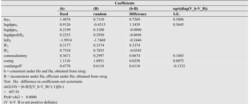
The gravity model in Equation 3.6 was first estimated using fixed effects regression and random effects regression (see results in Appendices A4.2 and A4.3 respectively). The hausman test was then applied to check whether the fixed effects model was more efficient than the random effects model. This would be true if the null hypothesis of no correlation between the individual effects and the regressors was rejected (see results in Appendix A4.4).
The Hausman test statistic shows that the null hypothesis was rejected, suggesting that the fixed effects (within) regression was more efficient than the random effects
regression. However, following Martinez-Zarzoso and Nowak-Lehmann (2003), time-invariant variables in the gravity model (such as distance, common language and common border) cannot be directly estimated with a fixed effects model because the inherent transformation wipes out such variables. Hence, the instrumental variables Generalized Method of Moments (GMM) regression was applied. The instrumental variables GMM regression is an efficient estimator of panel data models. It provides consistent estimates, addresses the endogeneity problem, and allows for efficient estimation in the presence of heteroskedasticity (Baum, Schaffer & Stillman, 2003).
4.3. Estimation Results and Discussion
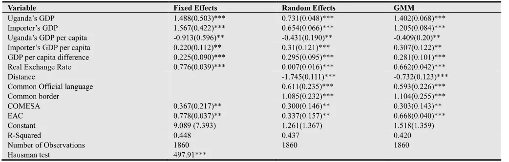
Table 4.1 summarizes the empirical results obtained from estimating Equation 3.6, using fixed effects (within) regression, random effects GLS regression and instrumental variables GMM regression.
Table 4.1. Empirical Results
Variable Fixed Effects Random Effects GMM
Uganda’s GDP 1.488(0.503)*** 0.731(0.048)*** 1.402(0.068)*** Importer’s GDP 1.567(0.422)*** 0.654(0.066)*** 1.205(0.084)*** Uganda’s GDP per capita -0.913(0.596)** -0.431(0.190)** -0.409(0.20)** Importer’s GDP per capita 0.220(0.112)** 0.31(0.121)*** 0.307(0.122)** GDP per capita difference 0.225(0.090)*** 0.295(0.095)*** 0.281(0.101)*** Real Exchange Rate 0.776(0.039)*** 0.007(0.016)*** 0.662(0.042)*** Distance -1.745(0.111)*** -0.732(0.123)*** Common Official language 0.611(0.235)*** 0.593(0.226)*** Common border 1.085(0.232)*** 1.104(0.255)*** COMESA 0.367(0.217)** 0.300(0.146)** 0.303(0.143)** EAC 0.778(0.037)** 0.337(0.157)** 0.668(0.040)*** Constant 9.089 (7.393) 1.261(1.367) 1.518(1.359)
R-Squared 0.448 0.437 0.420
Number of Observations 1860 1860 1860 Hausman test 497.91***
Dependent variable: Exports Standard errors in parentheses.
***, **, *: statistically significant at 1%, 5% and 10% levels respectively.
The effect of Uganda’s GDP was found to be positive and statistically significant at the 1 percent level in all estimated models, which is in line with theoretical expectation. This result suggests that Uganda’s GDP is a key determinant of the country’s capacity to export. A higher GDP means a higher production capacity which in turn translates into the ability of the economy to export more (supply side). This is consistent with the findings of Carrillo and Lee (2002) in their study of the effect of regional integration on both intra-regional and intra-industrial trade in Latin America in the period 1980-1997. Using the gravity model, these authors found the exporter’s GDP to be positive and statistically significant.
The effect of GDP of the importing country was found to be positive and statistically significant in all estimated models. This result suggests that a higher GDP for a trading partner country means a higher absorption capacity, implying that the trading partner country is able to import more (demand side). This is consistent with the findings of Orindi (2011). This author investigated the determinants of Kenyan
exports. He applied the gravity model on a sample of 25 trading partners from 1964 -2008. According to the study results, the importer’s GDP had a positive impact on the volume of bilateral trade between Kenya and its trading partners.
The effect of GDP per capita income difference was found to be positive and statistically significant at the 1 percent level in all estimated models. Its positive sign suggests that bilateral trade flows between Uganda and its trading partners are related positively to inter-country differences in the level
of technological advancement. Large technological
differences tend to promote bilateral trade between Uganda and its trading partners. Therefore, the Heckscher–Ohlin hypothesis was found to be valid. This result is consistent with the findings of Carrillo and Li (2002) whose study on trade blocs in Latin America found that the effect of GDP per capita income difference was negative in the case of the homogeneous product category, but was positive and statistically significant in the differentiated product category.
to be positive and statistically significant at the 1 percent level in all estimated models. This implies that the exchange rate had a significant effect on Ugandan exports during the period of study. The positive coefficient of exchange rate implies that Uganda’s exports depend on its currency devaluation. From the estimated results it is evident that 1% currency devaluation leads to, other things being equal, an increase of Uganda’s exports by 0.66%.
The effect of official common language was found to be positive and statistically significant in the random effects and GMM models, which is in line with the predicted theory. Sharing of an official common language promotes bilateral trade between Uganda and her trading partners. Melitz (2007) posits that the absence of a common language and the consequent presence of linguistic barriers can be a major obstacle to foreign trade. This result is consistent with the previous findings of Achay (2006), Eita and Jordaan (2007), Foroutan and Lant (1993), Martinez-Zarzoso and Nowak-Lehmann (2003) and Ram and Prasad (2000). In their empirical studies, these authors found a strong positive effect of the language variable and concluded that historical, cultural and colonial ties had a significant impact on the pattern of trade in their study samples.
The effect of common border was found to be statistically significant at the 1 percent level in the random effects and GMM models and in line with the predicted theory. Sharing a common border facilitates trade. Thus, countries with common frontiers with Uganda tended to have more bilateral trade. This result is consistent with the findings of Carrillo and Li (2002) whose empirical study on regional integration schemes in Latin American showed that adjacency had a very strong effect on the bilateral volume of trade.
The regression results show that the effect of Uganda’s GDP per capita income was negative and statistically significant at the 5 percent level in all estimated models. This implies that an increase in Uganda’s GDP per capita income raises the absorption capacity of the domestic market, resulting into lower exports. This result is consistent with the findings of Foroutan and Lant (1993). In a study on the effect of regional integration arrangements on trade in Sub-Saharan Africa, these authors found that a higher GDP per capita of an exporting country reduced the trade potential.
The effect of geographical distance was found to be negative and statistically significant at the 1 percent level in the random effects and GMM models, which is consistent with the theoretical expectation. These results provide strong support for the hypothesis that transportation costs are an important determinant of trade flows between Uganda and its trading partners. This implies that Uganda tended to trade more intensely with neighbouring countries, where transportation costs are lower, than those that are further apart. This result is consistent with the findings of Orindi (2011). This author assessed the role played by geographical proximity in determining Kenyan exports, and found that the geographical distance, among other factors, had a negative impact on the volume of trade between Kenya and its trading partners.
To assess the effect of COMESA on Uganda’s exports, a
comparison of the pre-COMESA period (1980-1993) with the post-COMESA period (1994-2010) was done through the
introduction of a
comesa
dummy variable. The effect ofthis dummy variable was found to be positive and statistically significant at the 5 percent level in all estimated models. Results from the GMM model show that exports from Uganda to COMESA members have grown by
approximately 35 percent
(
exp0.3− ×1)
100 since the formation of COMESA. This result suggests that the formation of COMESA has increased the propensity of Uganda to trade with COMESA member countries rather than with non-members. In a related study, Orindi (2011) found that Kenya’s exports were 12.5 times higher when the bilateral trade was between a COMESA member state than a non-COMESA member.Similarly, to assess the effect of the East African Community on Uganda’s exports, a comparison of the pre-EAC period (1980-1999) with the post-pre-EAC period
(2000-2010) was done through the introduction of an EAC dummy
variable. The effect of this dummy variable was also found to be positive and statistically significant at the 5 percent level in all estimated models. Results from the GMM model show that exports from Uganda to other EAC members have grown by approximately 40 percent since the formation of EAC.
5. Conclusion and Policy Implications
5.1. Conclusion
This study has examined the determinants of Uganda’s exports. An augmented trade gravity model was estimated using fixed effects (within) regression, random-effects GLS regression and instrumental variables GMM regression. The dataset was from 1980 to 2012. The results from the instrumental variables GMM model showed that Uganda’s GDP, importer’s GDP, importer’s GDP per capita, per capita GDP difference between Uganda and its trading partners, real exchange rate, official common language, and contiguity had a positive and statistically significant effect on Uganda’s exports. The study further, showed that the formation of COMESA and EAC had a significant positive effect on Uganda’s exports. On the other hand, Uganda’s GDP per capita and distance between Uganda and its trading partners had a negative and statistically significant effect on Uganda’s export flows.
5.2. Policy Implications
exports. These results are important for trade policy formulation in order to ensure that Uganda’s export potential
is exploited in order to enhance economic growth.
Table A4.1. Panel Unit Root Test Results
Variable Fisher test statistic Null: all series in panel contain unit root
IPS test statistic Null: all series in panel contain unit root
Export -0.735 (0.000)*** -4.422 (0.000)*** Importer’s GDP -0.823 (0.000)*** -14.556 (0.000)*** Uganda’s GDP 1.375 (0.000) *** -4.765 (0.000)*** Importer’s GDP per capita -1.345 (0.000)*** -14.224 (0.000)*** Uganda’s GDP per capita 2.223 (0.000) ** -6.654 (0.000)*** Real exchange rate -3.342 (0.000)*** -33.831 (0.000)***
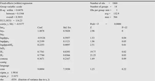
Table A4.2. Fixed Effects Model
Fixed-effects (within) regression Number of obs = 1860 Group variable: ccode Number of groups = 14 R-sq: within = 0.4476 Obs per group: min = 1
between = 0.1544 avg = 132.9
overall = 0.3033 max = 566
F(13,1833) = 114.23
corr(u_i, Xb) = -0.5377 Prob > F = 0.0000
lnxijt Coef. Std. Err. Z P>/Z/
lnyit 1.4878 0.5028 2.96 0
lnyjt
lngdppcit -0.9126 0.5957 1.53 0.04
lngdppcjt 0.2199 0.1121 1.96 0.05
lngdppcdiffijt 0.2253 0.0897 2.51 0.01 lnDij
IFit 0.7761 0.0393 19.77 0.02
IFjt 0.7784 0.0366 21.25 0.03
comesa 0.3671 0.2167 1.69 0.09
contig language
cons 9.0894 7.3930 1.23 0.22
sigma_u 1.9816 sigma_e 2.1671
rho .4554 (fraction of variance due to u_i)
Table A4.3. Random Effects Model
Random-effects GLS regression Number of obs = 1860 Group variable: ccode Number of groups = 14 R-sq: within= 0.4373 Obs per group: min = 1 between = 0.1841 avg = 132.9 overall = 0.4205 max = 566 Random effects u_i ~ Gaussian Wald chi2(13) = 1339.53 corr(u_i, X) = 0 (assumed) Prob > chi2 = 0.0000
lnxijt Coef. Std. Err. z P>/z/
lnyit 0.7310 0.0477 15.33 0
lnyjt 0.6710 0.0391 17.17 0
lngdppcit -0.4313 0.1903 -2.27 0.02
lngdppcjt 0.3100 0.1208 2.57 0.01
lngdppcdiffijt 0.2950 0.0950 3.11 0
lnDij -1.7469 0.1110 -15.74 0
IFit 0.0072 0.0156 0.46 0.02
IFjt 0.3374 0.1566 2.15 0.03
comlangoff 0.6110 0.2346 2.6 0
comesadummy 0.2997 0.1458 2.05 0.04
Border 1.0851 0.2324 4.67 0
cons 1.2610 1.3668 0.92 0.36
sigma_u 0.00 sigma_e 2.1671
Table A4.4. Hausman Test
Coefficients
(b) (B) (b-B) sqrt(diag(V_b-V_B))
fixed random Difference S.E.
lnyit 1.4878 0.7310 0.7569 0.5006 lngdppcit 0.9126 -0.4313 1.3439 0.5645 lngdppcjt 0.2199 0.3100 -0.0900
lngdppcdiffijt 0.2253 0.2950 -0.0696 lnDij -1.9914 -1.7468 -0.2446 IFit 0.3177 0.3374 0.3374 IFjt 0.7510 0.7855 -0.0345
comesadummy 0.3671 0.2997 0.0674 0.1603 contig 1.1110 1.0851 0.0258 0.0075 comlangoff 0.4778 0.6110 0.6110 -0.1332 b = consistent under Ho and Ha; obtained from xtreg
B = inconsistent under Ha, efficient under Ho; obtained from xtreg Test: Ho: difference in coefficients not systematic
chi2(10) = (b-B)'[(V_b-V_B)^(-1)](b-) = 497.91
Prob>chi2 = 0.0000
(V_b-V_B is not positive definite)
References
[1] Achay, L. (2006). Assessing Regional Integration in North Africa. National Institute of Statistics and Applied economics, Rabat, Morocco.
[2] Baltagi, B. (2005). Econometric Analysis of Panel Data. Third edition. Wiley. Baum, C. F., Schaffer, M. E. and Stillman, S. (2003). Instrumental Variables and GMM: Estimation and Testing. The Stata Journal, 3, 1-31. Working paper version: Boston College Department of Economics Working Paper No 545.
[3] Bergstrand, J. H. (1985). The Gravity Equation in International Trade: Some Microeconomic Foundations and Empirical Evidence. The Review of Economics and Statistics, 67, 474-481.
[4] Breitung, J. (2000). The Local Power of Some Unit Root Tests for Panel Data. Advances in Econometrics, 15, 161-177. [5] Carrillo, C. and Li, C. A. (2002). Trade Blocs and the Gravity
Model: Evidence from Latin American Countries. Working Paper, Department of Economics, University of Essex, UK.
[6] Chen, I-H. and Wall H. J. (1999). Controlling for Heterogeneity in gravity models of Trade. Federal Reserve Bank of St. Louis Working Paper 99-010A.
[7] Clarete, R., Edmonds, C. and Wallack, J. S. (2002). Asian Regionalism and its Effects on Trade in the 1980s and 1990s. Journal of Asian Economics, 14, 91-129
[8] Egger, P. (2000). A Note on the Proper Econometric Specification of the Gravity Equation. Economic Letters, 66, 25-31.
[9] Eita, J. H. (2008). Determinants of Namibian Exports: A Gravity Model Approach, University of Namibia, Namibia. [10] Eita, H. J. and Jordaan, A. C. (2007). South Africa’s Wood
Export Potential Using a Gravity Model Approach. University of Pretoria, Working Paper 2007-23, 1-24.
[11] Ekanayake, E. M., Mukherjee, A. and Veeramacheneni, B. (2010). Trade Blocks and the Gravity Model: A Study of Economic Integration among Asian Developing Countries. Journal of Economic Integration, 25(4), 627-643.
[12] Foroutan, F. and Lant, P. (1993). Intra-Sub-Saharan African Trade: Is it Too Little? Journal of African Economies, 2(1), 74-105.
[13] Frankel, J. (1997). Regional Trading Blocs and the World Economic System. Institute for International Economics, Washington D.C.
[14] Gani, A. (2008). Factors Influencing Trade Between Fiji And Its Asian Partners. Pacific Economic Bulletin Volume 23 Number 2, The Australian National University.
[15] Garnaut, R. (1994). Open Regionalism: Its Analytic Basis and Relevance to the International System. Journal of Asian Economics, 5(2), 273-90.
[16] Helpman, E. (1987). Imperfect Competition and International Trade: Evidence from Fourteen Industrial Countries. Journal of the Japanese and International Economies, 1(1), 62-81.
[17] Im, K. S., Pesaran, M. H. and Shin, Y. (2003). Testing for Unit Roots in Heterogeneous Panels. Journal of Econometrics, 115, 53-74.
[18] Kaberuka, W., Rwakinanga, E.T. and Tibesigwa, W. (2014). Is Export-led Growth Hypothesis Valid in Uganda? A Cointegration and Causality Analysis (1960-2010). Issues in Business Management and Economics, Vol.2 (4), pp060-073.
[19] Kihangire, D. (2005). The Effects of Exchange Rate Variability On Exports: Evidence from Uganda (1988-2001), International Trade, 0505013, EconWPA
[20] Kilimani, N. and Sebaggala, R. (2012) Trade Liberalization, Export a nd Import Growth: Evidence from Uganda
[22] Limão, N. and Venables, A. J. (1999). Infrastructure, Geographical Disadvantage and Transport Costs. Policy Research Working Paper 2257, World Bank.
[23] Linnemann, H. (1966). An Econometric Study of International Trade Flows. Amsterdam, Holland.
[24] Maddala, G. S. and Wu, S. (1999). A Comparative Study of Unit Root Tests with Panel Data and a New Simple Test. Oxford Bulletin of Economics and Statistics, 61, 631-652.
[25] Márquez-Ramos, L. (2007). Understanding The Determinants Of International Trade In African Countries: An Empirical Analysis For Ghana And South Africa. Instituto de Economía Internacional, Universitat Jaume I.
[26] Martinez-Zarzoso, I. & Nowak-Lehmann, F. (2003). Augmented Gravity Model: An Empirical Application to Mercosur-European Union Trade Flows. Journal of Applied Economics, 6(2), 291-316.
[27] Mátyás, L. (1997). Proper Econometric Specification of the Gravity Model. The World Economy, 20(3), 363-368.
[28] Melitz, J. (2007). Language and Foreign Trade. European Economic Review, 52, 667-699 London, UK.
[29] Musinguzi, P. (2002). Economic, Statistical Indicators and their relevance. Economic Policy Research Centre, Kampala. [30] Orindi M.N. (2011). Determinants of Kenyan Exports: A
Gravity Model Approach. Internationa Journal of Economic and Political Integration. Volume 1, Number 1.
[31] Pöyhönen, P. (1963). A Tentative Model for the Volume of Trade between Countries. Weltwirtschaftliches Archiv, 90(1), 93-100.
[32] Rahman, M. M. (2009). Australia’s Global Trade Potential: Evidence from the Gravity Model Analysis. In: Oxford Business and Economics Conference, 24-26 June, 2009, Oxford University, Oxford, UK.
[33] Ram, Y. and Prasad, B. (2000). Assessing Fiji’s Global Trade Potential using the Gravity Model Approach. Fiji, University of South Pacific.
[34] Roy, M. and Rayhan, I. (2011). Trade Flows of Bangladesh: A Gravity Model Approach, Economics Bulletin , Vol. 31 no.1 pp. 950 -959.
[35] Sohn, Chan-Hyun (2005). Does the Gravity Model Fit Korea’s Trade Patterns?
[36] Implications for Korea’s Trade Policy and North-South Korean Trade. Center for International Studies (CITS) Working Papers, Faculty of Economics, Yokahama National University. Statistics 67:474-481.
[37] Soloaga, I. and Winters, A. (1999). Regionalism in the Nineties: What effects on trade? Development Economic Group of the World Bank, mimeo.
[38] Taye, Y. T. (2009). Determinants of Ethiopia's Export Performance: A Gravity Model Analysis BKP Development Research & Consulting, Trade and Development Discussion Paper No. 01/2009.
[39] Tinbergen, J. (1962). Shaping the World Economy: Suggestions for an International Economic Policy. New York: The Twentieth Century Fund.
[40] Wei, S. J. (1996). Intra-National versus International Trade: How Stubborn are Nations in Global Integration? NBER, Working Paper 5531.