Shape design for polymer spin packs: modeling, optimization and validation

R E S E A R C H

Open Access

Shape design for polymer spin packs:

modeling, optimization and validation

Christian Leithäuser

_{, René Pinnau}

_{and Robert Feßler}

*_{Correspondence:}

[email protected] 1_{Fraunhofer Institute for Industrial} Mathematics ITWM, Kaiserslautern, Germany

Full list of author information is available at the end of the article

Abstract

A shape optimization approach for the design of cavities with a specified wall shear stress profile is presented. Applications are the design of spin pack geometries with low and uniform residence times and without dead spaces to prevent polymer degradation for sensitive materials. The optimization uses a Surrogate Model based on the Newtonian Stokes equation as a simplification. An indirect objective based on wall shear stress is used to improve the residence time. The results are then validated on a realistic spin pack with the Full Model based on the non-Newtonian

Navier–Stokes equation.

Keywords: Shape optimization; Computational fluid dynamics; Navier–Stokes equation; Non-Newtonian fluid; Approximate controllability

1 Introduction

Polymer spin packs are widely used for the production of synthetic fibers and non-woven materials. Polymer melt is extruded through a pipe into the spin pack geometry where it is first distributed along the whole cross-sectional area before it passes several layers of filter material and is finally spun into fibers by the spinneret plate which consists of a large number of very small nozzles. The whole spin pack is heated in order to prevent premature solidification of the melt. However, the influence of heat can lead to polymer degradation if the residence times are too long. For sensitive polymers with interesting properties this issue can be the limiting factor which prevents innovations due to the fact that spinning is not possible. This can be resolved by designing special spin packs with low residence time profiles. An important part in the spin pack design is the cavity which distributes polymer from the inlet pipe onto the whole cross-sectional area. This part of the geometry is in particular vulnerable for dead spaces and regions with slow flow velocities where degradation can take place. An indirect objective based on the wall shear stress is used to improve the residence time. The idea is that problematic regions usually occur in close proximity to the walls. In general a low wall shear stress coincides with a slow velocity zone close to the wall. On the other hand being able to design cavities with a sufficiently high level of stress throughout its wall is an effective tool against dead spaces and large residence times and thus against polymer degradation.

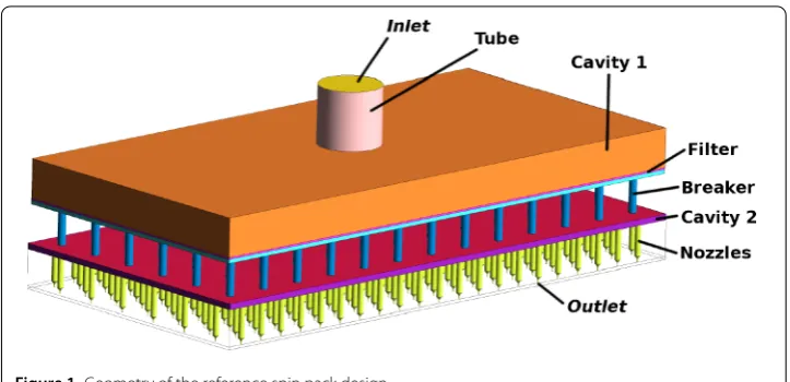
A spin pack is geometrically complex (see Fig.1) and most polymers are non-Newtonian. Typically, commercial simulation software is used for the simulation, which makes deriva-tive based shape optimization difficult to handle. Therefore, a surrogate model approach

Figure 1Geometry of the reference spin pack design

is used to optimize specific parts of the spin pack. The improved design is then validated with the complex model.

In Sect.2the two models are introduced: The Full Model is used for validation and is based on the non-Newtonian Navier–Stokes equation. It considers the whole geometry of the spin pack and pathlines are traced to evaluate the distribution of residence times. The Surrogate Model on the other hand is based on the Newtonian Stokes equation. It only considers the geometry of the spin pack cavity and wall shear stress is used as an indirect objective instead of residence time. The numerical approach for solving the shape optimization problem based on the Surrogate Model is derived in Sect.2.3and optimized cavities with uniform wall shear stress are presented in Sect.3.1. These cavities are then validated with the Full Model in Sect.3.2in a realistic setting.

Further numerical and theoretical results on the shape optimization of polymer spin packs can be found in [1–4]. Another interesting application of a similar problem is studied in [5,6]. The authors use shape optimization to design aorto-coronaric bypasses and use wall shear stress as an optimization criterion.

2 Methods

A typical spin pack used for fiber production is shown in Fig.1. Polymer enters through the Inlet, passes a short Tube and is distributed in Cavity 1 onto the Filter. Polymer passes the Breaker plate, which is basically a metal plate with a number of holes and its main purpose is to support the Filter. There is a second cavity (Cavity 2) before the material enters the Nozzles and is spun into fibers. The Nozzles consist of larger counterbores and then very small capillaries where the actual spinning takes place.

Table 1 Comparison between Full and Surrogate Model

Full Model Surrogate Model

PDE Navier–Stokes Stokes

Viscosity non-Newtonian Newtonian

Geometry whole spin pack Cavity 1 (Filter in boundary condition) Objective residence time wall shear stress

2.1 Full model: non-Newtonian Navier–Stokes

LetΩ⊂R3_{be the geometry of the spin pack. The flow is modeled using the stationary}

Navier–Stokes equation

–η(γ˙,T)

ρ u+ (u· ∇)u +

1

ρ∇p= F inΩ,

divu= 0 inΩ

(1)

with velocity u, pressurepand densityρ. The viscosityη(γ˙,T) depends on the shear rate ˙

γ and temperatureT. The temperature is assumed to be constant due to the controlled heating of the spin pack block. The source term F is set to zero everywhere except in the Filter where it is used to model a porous medium.

The shear rate is defined through the rate-of-deformation tensorD¯ by (see [7])

˙

γ =

1 2D¯:D¯

and the tensor is given by

¯

D= (∂iuj+∂jui)ij.

In order to model the viscosity a Cross model [8, Ch. 3.6] is used

η(γ˙,T) =H(T) η0

1 + (λγ˙)1–n (2)

with zero-shear-rate viscosityη0, time constantλand power-law indexn. The temperature

dependence is modeled through an Arrhenius law by

H(T) =exp

α

1

T –

1

Tα

(3)

with activation energyαand reference temperatureTα.

The Filter is modeled as a porous medium by adding a source term to the momentum equation [7]

F=Cfilter1

2ρ|u|u inΩfilter,

F= 0 inΩ\Ωfilter,

(4)

whereΩfilteris the filter part of the computational domain (see Fig.1). Typically the filter

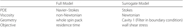
Figure 2Sketch of a geometry of the Surrogate Model with boundary partition

size as well as the number of pores per area are known. If one assumes equal flow rates per filter area it is possible to estimate the inertial loss coefficientCfilter from simulating the flow through a single pore. This assumption of uniform flow rates often holds because the Filter generates a significant pressure drop compared to its surroundings (cf. Fig.9).

Once the flow has been computed the residence time needs to be quantified. This is done by evaluating the residence time for a finite number of pathlines through the spin pack. Typically, we use the pathlines which end in the center of every capillary. The distribution of the residence times for the individual pathlines is used to compare the residence time distribution for different spin pack designs (cf. Fig.8). The residence time for a single pathline is computed in the following way: Let xout be a point on the outlet, for example

in the center of a capillary. The pathline is computed in reverse order by solving the ODE

˙

x(t) = –u(x),

x(0) = xout.

(5)

Note, that the sign in front of the velocity u is negative because the pathline is traced in reverse direction from outlet to inlet. The residence time for this individual pathline is then the timetat which the pathline reaches the inlet boundary.

2.2 Surrogate model: Newtonian Stokes

The goal is now to optimize the geometry such that the residence time distribution is short and with small deviations. To do this a number of simplifications leading to the Surrogate Model are introduced in the following.

Simplification 1: geometry. Instead of the full spin pack geometry depicted in Fig.1we only consider Cavity 1 for our Surrogate Model. This is signified because typically most of the residence time is spent in this cavity. The boundary decomposed into an inlet part

Γin_{, a wall partΓ}wall_{and an outlet partΓ}out_{(see Fig.2).}

Furthermore, the Filter sitting below the cavity is accounted for in the outlet boundary condition through a Darcy law [9, Eq. 1.2] which yields a relation between normal velocity and pressure:

nout(n·u) = –kout

η

p–pamb Lout onΓ

out ₍₆₎

with the porositynout, the permeabilitykout, the ambient pressurepamband the thickness

of the filterLout. It is important to consider the filter to get the correct velocity at the outlet. The filter typically generates a much higher pressure drop than the friction of the cavity. This basically results in equal flow rates throughout the whole outflow boundary.

viscosity. However, for most applications the shear thinning only occurs in the fine cap-illaries. The shear rates in the distributor cavities usually lie in the zero shear rate limit of the Cross model [8, Ch. 3.6] used to represent the viscosity (cf. Fig.6). Thus we use a constant viscosity

η(γ˙,T) =η= const,

which is independent of the shear rate.

Simplification 3: Stokes equation. Inertia does not play a role for the flow within the spin pack cavity, due to the high viscosity compared to the low velocities. Therefore, the Navier–Stokes equation can be replaced by the Stokes equation. The previous simplifica-tion lead to the following problem:

–ηu+∇p= 0 inΩ,

divu= 0 inΩ,

u= nu0 onΓin,

u= 0 onΓwall,

cout(n·u) +p= 0 onΓout,

n×u= 0 onΓout,

(7)

whereu0is a given inflow profile and n the outward pointing normal vector. With

cout=

noutηLout kout

and w.l.o.g.pamb= 0 the outflow boundary condition agrees with (6). The well-posedness

of the Stokes problem for these specific boundary conditions follows from [10, Prop. 4.7].

Simplification 4: wall shear stress objective. We use a cost function based on the wall shear stress as an indirect criterion to optimize the residence time. The reason is that the wall shear stress

σ=η|∇ ×u| onΓwall

can be directly evaluated from the flow in contrast to the residence time which involves an additional equation (5). Furthermore, when dealing with (5) it can happen that a pathline does not reach the end due to numerical reasons. This leads to discontinuities in the cost function and poses a problem for a gradient-based optimization approach.

This motivation leads to the following shape optimization problem:

min

Ω subject to (7)

J(Ω) =

Γwall

η|∇ ×u|–σd 2

ds, (8)

whereσdis a sufficiently high target wall shear stress.

2.3 Numerical shape optimization for the surrogate model

Let us derive the shape optimization approach for the Surrogate Model (8).

Geometry variations. Starting from any admissible domainΩ0⊂R3 of classC1,1 we

want to compute a gradient Vg which enables us to use a gradient descent approach for

solving the shape optimization problem. Knowing the gradient we can perform a descent step towards the domainΩ–sVg= (Id –sVg)(Ω0) for some step sizes> 0. Let

V1_:=V∈C1,1_R3_,R3_{; V|}

Γ₀in∪Γ₀out= 0 ,

Θ1:=

θ∈V1;θ_C1,1_(R3_,R3₎<1 2

.

(9)

We defineΩθ:= (Id +θ)(Ω0) which is again of classC1,1(see Remark1) and consider the

problem

–μu(θ) +∇p(θ) = 0 inΩθ,

divu(θ) = 0 inΩθ,

u(θ) = u0 onΓθin,

u(θ) = 0 onΓ_θw,

coutn·u(θ)+p(θ) = 0 onΓ_θout,

u(θ)×n= 0 onΓ_θout

(10)

with wall shear stress

σ(θ) =μ∇ ×u(θ)|Γ_θw=μ

∇ ×u(θ)·∇ ×u(θ)|Γ_θw. (11)

Remark1 Forθ ∈Θ1 _{it is implied by [11] that Id +θ :R}3_→R3 _{is an invertible (1,}

1)-diffeomorphism and thusΩθ= (Id +θ)(Ω0) is also of classC1,1. Then, a regularity

argu-ment similar to [12] would yield u(θ)∈[H2_(Ω

θ)]3, thusσ(θ)∈L2(Γθw) by the Trace Theo-rem [13, Thm. 8.7] and the objective (8) is well-defined. However, the focus of the current paper lies in the application and we will not derive the regularity result for our specific set of boundary conditions (10). We will rather use Assumption1and derive the gradient in a purely formal way.

Remark2 TheC1,1_{regularity of the domain can probably be relaxed further: If should}

suffice if the wall boundaryΓ_θwisC1,1_{. Therefore, sharp corners between inlet/outlet and}

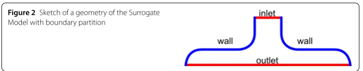
Figure 3Cavity A: Optimal distributor geometry for a target wall shear stress ofσd= 0.1

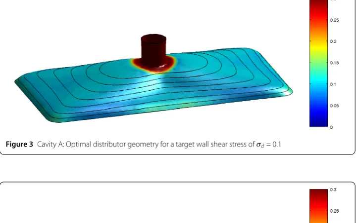
Figure 4Cavity B: Optimal distributor geometry for a target wall shear stress ofσd= 0.2

Sensitivity analysis. In order to compute the sensitivity we follow the optimize then dis-cretize approach. Therefore, we need to differentiate the cost functional and the partial differential equation with respect to the shape, which requires the existence of the cor-responding shape derivatives. However, the focus of this part is to derive a numerical method suited to solve the industrial problem, therefore, we omit the existence and regu-larity proofs for the shape derivatives and make the following assumption:

Assumption 1 Assume the existence of u(θ)∈H2_(Ω

θ,R3), p(θ)∈H1(Ωθ) andσ(θ)∈ L2_(Γw

θ ) for θ ∈Θ1 and the existence of the shape derivatives u(Ω0; V)∈H2(Ω0,R3), p(Ω0; V)∈H1(Ω0) andσ(Γ0; V)∈L2(Γ0w) for V∈V1.

Definition 1(Shape derivative [14]) Form≥1 lety(sV)∈Hm_{((Id +sV)◦Ω}

0) fors∈R

sufficiently small. Then, the shape derivative ofyin direction V is defined by

y(Ω0, V) :=lim s→0

1

s

y(sV)◦(Id +sV) –y(0)–∇y(0)·V∈Hm–1(Ω0).

Furthermore, the shape derivative ofyrestricted to the boundary is

y(Γ0, V) :=y(Ω0, V)|Γ0+∂ny(0)(n·V)∈H

m–3_2(Γ 0).

For details and a more general definition of the shape derivatives we refer to [14].

The cost function

J(Ωθ) =

Γ_θw

σ(θ) –σd 2

ds (12)

is differentiated with respect toθ. The derivative of a boundary integral is given in [14]. Applying this to (12) yields for the derivative in direction V∈V1

dJ(V) =dJ(Ωθ)

dθ (V)

=

Γ₀w

σ(θ) –σd 2

|Γ_θw

(Γ0; V)ds+

Γ₀w

κ(n·V)σ(0) –σd 2

ds, (13)

whereκdenotes the curvature (see [14]).

We assume that the wall shear stressσ(0) is nonzero on the wall boundaries. For geome-tries with one inflow and one outflow this is fulfilled automatically. For more complicated geometries we may have to exclude neighborhoods of stagnation points from the wall boundaries. If this assumption holds, we can derive the shape derivative ofσ(θ) by

σ(Γ0; V) =

μ

2√∇ ×u(0)· ∇ ×u(0)

∇ ×u(θ)· ∇ ×u(θ)|Γ_θw

(Γ0; V)

= μ

2

σ(0)∇ ×u(0)·

∇ ×u(θ)|Γ_θw

(Γ0; V)

= μ

2

σ(0)∇ ×u(0)·

∇ ×u(Ω0; V)

|Γ₀w+ (n·V)∂n

∇ ×u(0). (14)

Thus (13) becomes

dJ(V) =

Γ₀w

2μ2σ(0) –σd

σ(0) ∇ ×u(0)· ∇ ×u _(Ω

0; V)ds

+

Γ₀w

2μ2σ(0) –σd

σ(0) ∇ ×u(0)·∂n

∇ ×u(0)(n·V)ds

+

Γ₀w

κσ(0) –σd 2

We need to deal with the first term of (15) which contains the shape derivative u(Ω0; V).

As shown in [15] the shape derivative (u(Ω0; V),p(Ω0; V)) can be computed as the

solu-tion of

–μu(Ω0; V) +∇p(Ω0; V) = 0 inΩ0,

divu(Ω0; V) = 0 inΩ0,

u(Ω0; V) = 0 onΓ0in,

u(Ω0; V) = –(n·V)∂nu(0) onΓ₀w,

coutn·u(Ω0; V)

+p(Ω0; V) = 0 onΓ0out,

u(Ω0; V)×n= 0 onΓ0out.

(16)

We introduce the adjoint variables (v,q) as solutions of the adjoint Stokes problem

–μv+∇q= 0 inΩ0,

divv= 0 inΩ0,

v= 0 onΓ₀in,

n·v= 0 onΓ₀w,

v×n= 2μσ–σd σ

∇ ×u(0) onΓ₀w,

cout(n·v) +q= 0 onΓ₀out,

v×n= 0 onΓ₀out.

(17)

Then, we can derive through integration by parts

0 =

Ω0

–μu(Ω0; V) +∇p(Ω0; V)

·vdx+

Ω0

divu(Ω0; V)q dx

=

Ω0

μ∇ ×u(Ω0; V)· ∇ ×vdx+

Γ0

μ∇ ×u(Ω0; V)·(v×n)ds

–

Ω0

p(Ω0; V)divvdx+

Γ0

p(Ω0; V)n·vds

+

Ω0

u(Ω0; V)· ∇q dx–

Γ0

n·u(Ω0; V)q ds

= –

Ω0

μu(Ω0; V)·vdx+

Γ0

μ∇ ×u(Ω0; V)·(v×n)ds

–

Γ0

μu(Ω0; V)×n

· ∇ ×vds+

Γ0

ηoutn·u(Ω0; V)n·vds

+

Ω0

u(Ω0; V)· ∇q dx–

Γ0

ηoutn·u(Ω0; V)n·vds

=

Γ0

μ∇ ×u(Ω0; V)·(v×n)ds–

Γ0

μu(Ω0; V)×n

which yields the identity

Γ₀w

2μ2σ(0) –σd

σ(0) ∇ ×u(0)· ∇ ×u _(Ω

0; V)ds

= –

Γ₀w

μ∂nu(0)×n

· ∇ ×v(n·V)ds. (19)

Plugging this identity into (15) yields

dJ(V) = –

Γ₀w

μ∂nu(0)×n

· ∇ ×v(n·V)ds

+

Γ₀w

2μ2σ(0) –σd

σ(0) ∇ ×u(0)·∂n

∇ ×u(0)(n·V)ds

+

Γ₀w

κσ(0) –σd 2

(n·V)ds. (20)

Discretization. Following the optimize then discretize approach we us Taylor–Hood fi-nite elements to discretize the partial differential equations. The implementation is done in COMSOL Multiphysics.

Using the spaceV1_{for the numerics is not reasonable because it would require the}

pro-jection of the gradient into a high order Sobolev space which has an embedding intoC1,1_.

For our approach numerical results have shown thatH2_{-regularity of the gradient is}

suf-ficiently smooth, even though there is no embedding fromH2_intoC1,1_{. Therefore, in the}

discrete problem the spaceV1_{is replaced with}

H2 k:=

V∈H2Ωk,R3

; V|Γ_kin∪Γ_kout= 0 .

The discrete gradient is then obtained by projectingdJ(ν) intoH2

kby solving

(Vk,ν)H2_(Ω

k)=dJ(ν) for allν∈H 2

k, (21)

with Vk∈H2kwhere (·,·)H2_(Ω

0)denotes the scalar product inH

2_.

Gradient descent method. In the last section the gradient of the cost function was de-rived, which enables us to apply the gradient descent method to solve the shape optimiza-tion problem. A small change of notaoptimiza-tion is performed: In the following letΩkdenote the

domain of iterationkof the gradient descent algorithm and the gradient atΩkis denoted

by Vk. Using this notation the gradient descent method is given in Algorithm1. An Armijo

rule (cf. [16]) was used to determine the step length, whereβ,γ > 0 are proper constants. Note, that theL2_{-norm was used for step size control and stopping criterion. However,}

with the state space Vk∈H2k theH2-norm might be a better choice. We do not expect

that this would significantly change the results, but it might improve the convergence.

Moving the mesh. This section explains how the mesh is moved and what smoothing operatorST is used. An important question is how the shape deformationΩk+1= (Id – βj_V

k)(Ωk) is carried out. In the current setup we work with a triangulationTkofΩkby

tetrahedral elements. Then we move every vertexξ∈Tkto (Id –βjVk)(ξ) to generate the

new meshTk+1. In the case that any elements of the mesh are inverted we regenerateTk+1

Algorithm 1L2_{Shape Optimization (3D)}

1: Let the target wall shear stressσdand initial domainΩ0⊂R3be given. Setk= 0.

2: loop

3: Solve Stokes equation (10) for (u,p) onΩk.

4: Solve adjoint Stokes (17) for (v,q) onΩk.

5: Solve: Find Vk∈H2kwith (Vk,ν)H2_(Ω

k)=dJ(ν) for allν∈H 2 k.

6: ifVkL2_(Ω

k)≤εtolV0L2(Ω0)then 7: return

8: end if

9: j←0

10: whileJ(Ωk) –J((Id –βjVk)(Ωk)) <γ βjVk2_L2_(Ω

k)do

11: j←j+ 1

12: end while

13: Ωk+1= (Id –βjVk)(Ωk)

14: Smooth the mesh:Ωk+1←ST(Ωk+1)

15: k←k+ 1

16: end loop

However, a problem is that the mesh tends to loose smoothness and becomes irregular. This has the effect that already after very few iterations the gradient fails to provide a proper descent direction and the algorithm stops. This is a common problem in shape optimization, as discussed in [15]. To overcome this we apply a smoothing operatorS_T to the deformed mesh. The operator is applied to the boundary mesh and is able to recover a boundary shape with more regularity. Of course the in- and outflow boundaries are not effected by the smoothing. We use the implementation [17] which relies on [18]. Using the smoothing step leads to a good quality of the gradient and a stable gradient descent algorithm. See [2, Theorem 6.5] where we have shown the existence of an optimal control for a similar problem.

3 Results and discussion

In the following Algorithm1bases on the Surrogate Model is used to compute optimized cavities. These cavities are then tested with the Full Model. A dimensionless setting was used for the optimization, while the validation was done in a realistic setting with units given later.

3.1 Shape optimization based on the surrogate model

With the presented shape optimization approach it becomes possible to design cavities with a specific wall shear stress profile. Figures3and4show two cavities with a constant target wall shear stress ofσd= 0.1 andσd= 0.2, respectively. Full details on the setup for

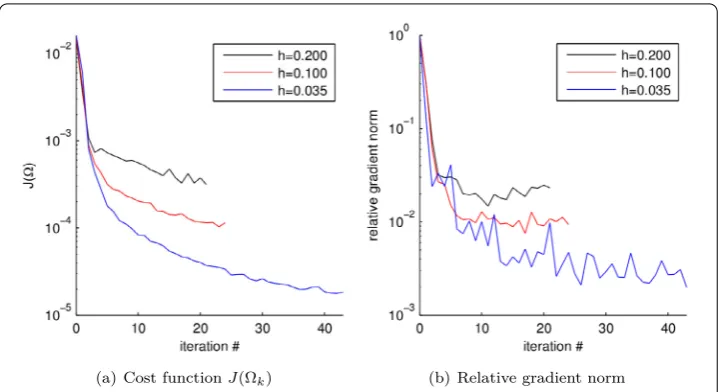
Figure 5Convergence of the cost functional and the relative gradient norm using Algorithm1to compute Cavity A with different mesh sizesh

(cf. [19]). However, for our current applications this simple gradient descent approach has proven to be sufficient.

3.2 Validation based on the full model

While we have seen that the proposed shape optimization algorithm is able to design dis-tributor cavities with a very uniform wall shear stress it remains to show how these cavi-ties perform in a realistic application. In this section a typical reference spin pack design is compared to optimized designs. The reference design is shown in Fig.1. In the reference design Cavity 1 is just a flat rectangular-shaped space which is quite common for many spin packs still in use today. However, this space is very vulnerable to dead spots which can then encourage polymer degradation due to long residence times. Therefore in the following Cavity 1 will be replaced by the two optimized cavities computed in Sect.3.1 and results regarding residence time, wall shear stress and pressure drop are compared.

The commercial CFD software ANSYS® Fluent is applied to model the spin pack in this validation step.

Geometric setup, data and boundary conditions. The geometry of our reference spin pack with 279 nozzles is depicted in Fig.1. The spacial dimensions of the bounding box are: 286 mm x 146 mm x 96 mm (length x width x height). In the following three geometries are compared:

• Reference: The reference design from Fig.1.

• Optimized A: Cavity 1 of the reference design replaced with the optimized cavity from Fig.3(Cavity A).

• Optimized B: Cavity 1 of the reference design replaced with the optimized cavity from Fig.4(Cavity B).

These spin pack geometries can be seen from Fig.7.

Figure 6Viscosity of Polypropylene (PP) from Springer Handbook of Condensed Matter and Materials Data [20, Fig. 3.3-13] and fitted cross model with coefficients from Table2

Table 2 Cross model coefficients to model the viscosity of Polypropylene (PP) in Fig.6

zero-shear-rate viscosity η0 6421.8 Pa s

time constant λ 0.6304 s

power-law index n 0.4276

activation energy α 3742.5 K

reference temperature Talpha 473.16 K

ρ= 900 kg m–3 _{[20, Table 3.3-5] and a constant temperature ofT = 237}◦_{was used. The}

inertial resistance coefficient for the filter was set toCfilter= 1e + 13 m–1. For the applied mass flow rate this results in a pressure drop of about 5 bar through the filter. At the inlet a constant mass flow of 41 kg h–1was set. The velocity profile itself is then determined by the solver. At all outlets of the 279 capillaries an outflow boundary condition with zero ambient pressure was set. At the boundaries of the porous Filter a slip condition was used because friction is already represented in the source term. No-slip boundary conditions were used on all other boundaries.

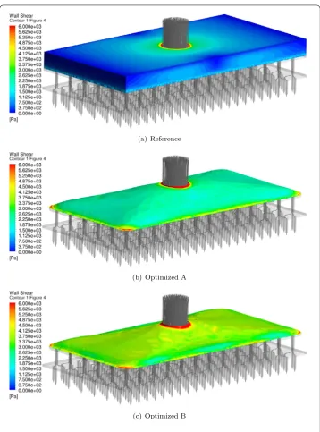
Numerical results. Simulations for the given setup for the Full Model were performed with ANSYS® Fluent for the reference design, as well as for the two optimized designs (Optimized A and Optimized B). Results for the wall shear stress in Cavity 1 are shown in Fig.7. The wall shear stress in the reference design Fig.7(a) is very low, especially in the outer regions which indicates stagnation zones. The wall shear stress for the optimized designs in Fig.7(b) (Optimized A) and Fig.7(c) (Optimized B) is significantly higher. As intended by the shape optimization approach the wall shear stress is very uniform. This shows that the shapes obtained with the Surrogate Model are still valid with the Full Model. Note, that the absolute level of the wall shear stress differs between the optimization step (Figs.3and4) and the validation step (Fig.7). The reason is that the optimization step was carried out in a dimensionless setting, while typical real world values were used for the validation step.

Figure 7Comparison of the wall shear stress in Cavity 1 for the three spin pack designs. Furthermore, the 279 pathlines which end in the center of each capillary are shown

Figure 8Comparison of the residence times measured along 279 representative pathlines for the three geometric design variations

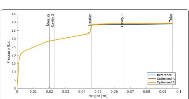
Figure 9Pressure plotted vs. the height of the spin pack. There are only minimal differences in pressure between the three geometric cases

optimized designs show a significant reduction of the residence time in Cavity 1 as well as for the total time. Also the spread of residence time was greatly reduced.

4 Conclusion

The presented shape optimization approach is able to generate cavities with specific wall shear stress profiles. This has proven to be an effective tool in the optimization of poly-mer spin packs and filter devices for sensitive applications. It is now possible to design geometries without dead spaces and with short and more uniform residence times. The optimization approach uses the Surrogate Model as a simplification. However, the valida-tion has shown that the cavities optimized with the simplified model are still valid in the more realistic setting of the Full Model. We have further seen that cavities with optimized wall shear stress lead to reduced and more uniform residence times within the spin pack while the increase in pressure stays minimal. Our ongoing and future research on this matter includes the use of parameterized geometries to improve the regularity as well as optimizing the residence time directly without the use of wall shear stress as an indirect criterion.

Acknowledgements Not applicable.

Funding

This work was supported by the German Federal Ministry of Education and Research (BMBF) grant no. 03MS606F and by the German Federal Ministry for Economic Affairs and Energy (BMWI) grant no. IGF 17629 N.

Abbreviation Not applicable.

Availability of data and materials

All spin pack geometries depicted in Fig.7are provided.

Competing interests

The authors declare that they have no competing interests.

Authors’ contributions

All authors read and approved the final manuscript.

Author details

1_{Fraunhofer Institute for Industrial Mathematics ITWM, Kaiserslautern, Germany.}2_{TU Kaiserslautern, Kaiserslautern,}

Germany.

Publisher’s Note

Springer Nature remains neutral with regard to jurisdictional claims in published maps and institutional affiliations.

Received: 12 February 2018 Accepted: 27 November 2018 References

1. Leithäuser C, Feßler R. Characterizing the image space of a shape-dependent operator for a potential flow problem. Appl Math Lett. 2012;25(11):1959–63.

2. Leithäuser C. Controllability of Shape-dependent Operators and Constrained Shape Optimization for Polymer. Distributors [PhD Thesis]. Kaiserslautern: TU; 2013.

3. Leithäuser C, Pinnau R, Feßler R. Approximate controllability of linearized shape-dependent operators for flow problems. ESAIM Control Optim Calc Var. 2017;23(3):751–71.

4. Leithäuser C, Pinnau R. The production of filaments and non-woven materials: the design of the polymer distributor. In: Math for the digital factory. Berlin: Springer; 2017. p. 321–40.

5. Quarteroni A, Rozza G. Optimal control and shape optimization of aorto-coronaric bypass anastomoses. Math Models Methods Appl Sci. 2003;13(12):1801–24.

6. Rozza G. On optimization, control and shape design of an arterial bypass. Int J Numer Methods Fluids. 2005;47(10–11):1411–9.

7. ANSYS®Fluent, Release 18.1, Help System, Fluent Guide;.

8. Kennedy P, Zheng R. Flow analysis of injection molds. Munich: Hanser Verlag; 2013. 9. Nield DA, Bejan A. Convection in porous media. New York: Springer; 2006.

10. Ern A, Guermond JL. Theory and practice of finite elements. vol. 159. Berlin: Springer; 2004.

11. Simon J. Differentiation with respect to the domain in boundary value problems. Numer Funct Anal Optim. 1980;2(7):649–87.

13. Wloka J. Partial differential equations. Cambridge: Cambridge University Press; 1987.

14. Sokolowski J, Zolesio JP. Introduction to shape optimization: shape sensitivity analysis. vol. 16. Berlin: Springer; 1992. 15. Mohammadi B, Pironneau O. Applied shape optimization for fluids. USA: Oxford University Press; 2001.

16. Alt W. Nichtlineare Optimierung. Wiesbaden: Vieweg; 2002.

17. Kroon DJ. Smooth Triangulated Mesh.http://www.mathworks.com/matlabcentral/fileexchange/ 26710-smooth-triangulated-mesh(2010).

18. Desbrun M, Meyer M, Schröder P, Barr AH. Implicit fairing of irregular meshes using diffusion and curvature flow. In: Proceedings of the 26th annual conference on computer graphics and interactive techniques. New York: ACM; 1999. p. 317–24.