R E S E A R C H
Open Access
Towards end-to-end speech recognition
with transfer learning
Chu-Xiong Qin
1,2, Dan Qu
1*and Lian-Hai Zhang
1Abstract
A transfer learning-based end-to-end speech recognition approach is presented in two levels in our framework. Firstly, a feature extraction approach combining multilingual deep neural network (DNN) training with matrix factorization algorithm is introduced to extract high-level features. Secondly, the advantage of connectionist temporal classification (CTC) is transferred to the target attention-based model through a joint CTC-attention model composed of shallow recurrent neural networks (RNNs) on top of the proposed features. The experimental results show that the proposed transfer learning approach achieved the best performance among all end-to-end methods and could be comparable to the state-of-the-art speech recognition system for TIMIT when further jointly decoded with a RNN language model.
Keywords:Speech recognition, End-to-end, Transfer learning
1 Introduction
A traditional speech recognition system can be divided into several modules such as acoustic models, language models, and decoding. The design of modularization re-lies on many independent assumptions, and even a trad-itional acoustic model is trained in a frame-wise way which depends on Markov assumptions. To eliminate all potential assumptions from an entire speech recognition system and to build a single model optimized in a se-quence level, the end-to-end method was introduced in the area and has become popular recently [1–3]. With the booming development of deep learning methods and under the help of high-performance graphic processing units, end-to-end approaches have been successfully im-plemented in speech recognition. Multiple convolutional and recurrent layers are added in to build an integrated network which acts both as an acoustic model and a lan-guage model, directly mapping speech inputs to tran-scriptions. Specifically, there are two major end-to-end methods for speech recognition, namely connectionist temporal classification (CTC) and attention-based model.
In most speech recognition tasks, performance of trad-itional systems still triumph end-to-end approaches [4– 7]. Many published results have shown that the perform-ance gap between them shrinks with greater amount of training data. For example, success of Baidu’s Deep Speech [4, 8] and Google’s Listen, Attend, and Spell models [9,10] demonstrated that an end-to-end system benefits in high-resource conditions. A key reason be-hind this conclusion is that current end-to-end models are trained in a data-driven way. All parameters in end-to-end models are updated by computations of gra-dients which are easily affected by structures of net-works, so theoretically there is no expert knowledge involved during training. However, end-to-end systems still fail to reach to a state-of-the-art performance even when they are trained with large corpora such as LibriS-peech and Switchboard which have thousands of hours of training data. We assume that end-to-end models suf-fer insufficient training in most cases. In order to neutralize the problem, different variants of networks have been introduced into both CTC and attention-based models. Complex encoders composed of convolu-tional neural networks (CNN) are introduced in order to exploit local correlations in speech signals [11–13]. Also joint architectures such as recurrent neural networks (RNNs) combined with conditional random field (CRF) [14], and joint CTC-attention systems [15] are proposed.
* Correspondence:[email protected]
1National Digital Switching System Engineering and Technological R&D Center, Zhengzhou, China
Full list of author information is available at the end of the article
They both take advantages of each sub-model and bring more explicit and strict constraints to the whole model. Although such researches above do improve automatic speech recognition (ASR) performances of end-to-end speech recognition systems, we believe it is hard to find a trade-off strategy between improving complexities of networks and solving low-resource limitations. Though introducing complex computational layers into the model could exploit better correlations in both time and frequency domain, a model with much more parameters would also be harder to train. For end-to-end models, the way of data-driven training without expert know-ledge involved becomes a bottleneck.
We propose a transfer learning-based approach that aims to solve the problem with limited speech resource under end-to-end architecture. Previous work has demon-strated that deep learning models across different lan-guages are transferable [16, 17], and multi-task learning (MTL) is helpful for end-to-end training [14, 15]. In our research, transfer learning is implemented in two levels. Firstly, we extract high-level representations of target speech leveraging a multilingual pre-trained network. We then use nonnegative matrix factorization (NMF) instead of a bottleneck layer to extract high-level speech features, expecting to make the most of nonlinearities of deep neural network (DNN) without breaking their structures during training. Secondly, we build a joint CTC-attention end-to-end model on top of the extracted high-level fea-tures in order to improve robustness through shared training and joint decoding. We use only a shallow bi-directional RNN instead of a complex encoder in [18]. To exploit as much similarities from multiple data sources as possible, both the end-to-end models and multilingual DNNs are trained in a phone level.
Our paper is organized as follows. We describe out method in Section2 and Section3. In Section 2, we de-scribe our high-level feature extraction approach with data augmentation. In Section3, we introduce the joint CTC-attention model. We introduce our experimental setup and analyze our experimental results in Section4. At the last section, we provide our conclusions.
2 High-level feature extractions with data augmentation
Although an ideal end-to-end ASR system aims to build a model mapping from raw inputs to phone/character se-quences, systems using transformed features like fMLLR (feature-space maximum linear logistic regression) fea-tures or introducing complex encoders before RNN tend to perform better compared with those using raw waves or classical features in many tasks [6,11, 13,19]. We as-sume that transformation in frequency domain could make up for some shortages of limited resource.
Classical features such as MFCC or filterbank are only low-level phonetic representations. It requires deep non-linear transformations for such features in end-to-end models. Unlike classical acoustic features, high-level fea-tures are often extracted through DNN and are demon-strated to be high-level semantic representations.
2.1 Multilingual training with maxout and dropout In order to further alleviate the problem caused by lim-ited training resource, we use multilingual training in feature extraction as data augmentation. Although multilingual training is trivial to directly apply on RNNs, it is useful to exploit acoustic similarities from shared layers. We believe that extracting multilingual-based high-level features is an effective way to embed general acoustic knowledge into end-to-end models. Inspired by [15, 18] and our previous work [20], we propose two types of feature extractors for end-to-end systems.
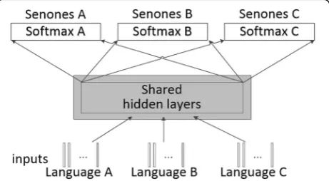
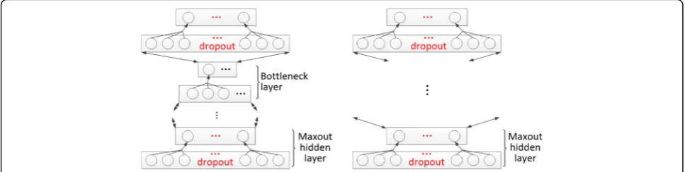
We first train several target independent DNNs with shared hidden layers using multiple language resources. An example for DNN with multilingual training is shown in Fig. 1. Instead of restricted Boltzmann ma-chine (RBM), we use maxout activation with dropout training to avoid over-fitting problem and to capture better generalities. Three different languages are trained simultaneously, and their senones corresponding to in-puts are considered as supervisions. Two different sche-matic structures of hidden layers are shown in Fig. 2. Figure 2a shows a maxout-dropout hidden structure with a bottleneck layer, and Fig. 2b shows a maxout-dropout hidden structure without a bottleneck layer.
For each hidden layer except for the bottleneck layer, activation outputs are described as follows:
xl
t ¼ultDt;1≤l≤L;1≤t≤T ð1Þ
whereultis the activation outputs of layerlfortth frame. Dt is the same sized vector filled with binary elements
each of which represents whether the corresponding
unit stays non-updated or not. ⊗ stands for the dot product operation.
DenoteIas actual output number of units in each hid-den layer and suppose the pooling size is 3 with no over-lapping, then there are 3I units before max pooling. Denote those units as a vectorvlt,vlt ¼ ½vltð1Þ;…;vltðiÞ;… ;vl
tð3IÞð1<i<3IÞ. The actual maxout outputs are cal-culated as follows:
ul
tð Þ ¼i max vltð3i−2Þ;vltð3i−1Þ;vltð Þ3i
;1≤i≤I ð2Þ
For the first type, we set bottleneck layers to obtain traditional bottleneck features for end-to-end multilin-gual training. We do not apply dropout for the bottle-neck layer, considering that dropout could do harm to a layer which does not have too many units. Besides, DNNs are supervised by tied triphone units that are gen-erated by Gaussian mixture models (GMM) while inputs are classical low-level acoustic features.
It has been demonstrated that lower layers of a DNN are transferable to new classification tasks. For the multilingual pre-trained network that includes a bottle-neck layer, we transfer all layers below the bottlebottle-neck layer to the target bottleneck DNN. Then, we stack a hidden layer and a softmax layer on top of them to build the target DNN. For the pre-trained network without setting a bottleneck layer, we propose a very different ap-proach. This is motivated by a hypothesis that setting a bottleneck layer degrades the classification accuracy of a DNN, which is also harmful to the bottleneck features themselves. Therefore, we would like to extract low-dimensional features from DNN without bottleneck layers. We first transfer all parameters below the last hidden layer from Fig. 2b and add a new softmax layer with random parameters to initialize the target DNN, and then we fine-tune the whole target DNN. Such adapt training without breaking the structure during training enables us keep maximum nonlinearity for later processing.
2.2 High-level feature extractions using NMF
We need to do dimensionality reduction to extract fea-tures since a high-dimensional vector output from a hid-den layer contains many redundant values. Although this approach is in a two-step fashion, it would be better if the dimension-reduction were associated closely with the DNN so that the features could benefit most from supervision of phone/state indirectly. Since it is obvious that weight matrices in DNN determine how vectors of hidden representations are formed, we apply matrix factorization algorithms on weight matrix of DNN in-stead of directly implementing naive dimensionality re-duction algorithms on hidden outputs.
In this paper, we adopt convex nonnegative matrix factorization (CNMF) to extract high-level features.
NMF has advantages over singularly valuable decompos-ition (SVD) and principal components analysis (PCA) in this problem. SVD and PCA are mathematically equivalent when dealing with the dimensionality reduction problem [21]. When using SVD to compact networks [22], we only select a certain amount of singular values. Both left-singular matrix and right-singular matrix contain much nonlinearities of the target weight matrix. Therefore through ignoring some component from matrices to form a linear project layer would cause certain losses. Compared with SVD, almost all NMF algorithms require at least one matrix to be nonnegative. Therefore, the target matrix could be defined as weighted sum of columns in the base matrix. Note that this is a very important constraint be-cause this makes the coefficient matrix much less import-ant when we only wimport-ant to keep the basic part of the original matrix. This explains why NMF is more interpret-able than SVD and PCA when dealing with our problem. NMF is demonstrated to discover base features embedded in matrices [23] which we believe would be useful for limited-resource condition. Additionally, we do not use ori-ginal NMF because it only deals with nonnegative values which are not the case for weight matrices of DNN.
As a variant of NMF, CNMF not only has no hard bound for values, but also restrict the base matrix to be
convex combinations of columns in the target matrix. Assuming the target weight matrix X has a size of N×
M, it is factorized into a base matrix F (with a size of
N×R) and a coefficient matrixG(with a size ofR×M). We first useK-means to initialize CNMF, as described in [23], to obtain cluster indicators H= (h1,…,hk). h1, …,
hk are vectors containing binary values. Then, we
initializeGwith
Gð Þ0 ¼Hþ0:2E; ð3Þ
where E is an identity matrix. F is initialized as cluster centroids:
F¼XHD−1
n ; ð4Þ
whereDn= diag(n1,…,nk) and n1, …, nkare numbers of
classes. CNMF defines F to be linear combinations of
columns of X, which isF=XW. Therefore we get Wð0Þ
¼HD−1
n according to this constraint and (4). Then G
andWare updated as follows until convergence:
Gik
ffiffiffiffiffiffiffiffiffiffiffiffiffiffiffiffiffiffiffiffiffiffiffiffiffiffiffiffiffiffiffiffiffiffiffiffiffiffiffiffiffiffiffiffiffiffiffiffiffiffiffiffiffiffiffiffiffiffiffiffiffiffiffiffiffiffiffiffiffiffiffiffiffiffiffi
XTX
þW
h i
ikþ GW
TXTX−W
ik
XTX
−W
ikþ GWT XTX
þW
h i
ik
v u u u
t →Gik
Wik
ffiffiffiffiffiffiffiffiffiffiffiffiffiffiffiffiffiffiffiffiffiffiffiffiffiffiffiffiffiffiffiffiffiffiffiffiffiffiffiffiffiffiffiffiffiffiffiffiffiffiffiffiffiffiffiffiffiffiffiffiffiffiffiffiffiffiffiffiffiffiffiffi
XTX
þG
h i
ikþ X TX
−WGTG
ik
XTX
−G
ikþ XTX
þWGTG
h i
ik
v u u u
t →Wik
8 > > > > > > > > < > > > > > > > > :
ð5Þ
where (⋅)− and (⋅)+
denotes generalized {1}-inverse and Moore–Penrose pseudoinverse respectively. After train-ing, the base matrix F and the coefficient matrix G are obtained.
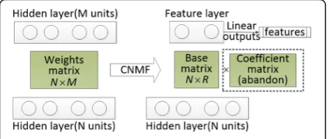
Figure 3 shows high-level feature extraction through applying CNMF on a specific hidden layer. Weights matrix of a certain hidden layer is factorized into two matrices following the above process. We abandon G and setFto be the weight matrix of the new feature ex-traction layer. The new layer is functionally similar to bottleneck layer, except that we calculate the features without the bias variable:
f¼ FTu¼WTXTu ð
6Þ
We can see from (6) that the features are transformed on original hidden outputsXTu viaWT. Note thatWis trained with original weight matrix X involved and act as a matrix for dimensionality reduction; therefore, we believe that our high-level features could capture multi-lingual acoustic similarities and at the mean time alleviate sparse problem caused by limited resource.
3 Joint CTC-attention
In this section, we will describe the end-to-end model of our transfer learning approach on top of our high-level features. Following the structure in [18], our end-to-end architecture is a joint CTC-attention model which consists of a shared encoder and a joint decoder. Our design is to transfer mono-tonic constraint from CTC to the target attention-based model to improve accuracy through joint modeling.
3.1 Joint training with shared encoder
The network for feature extraction could also be consid-ered as intermediate supervision for our end-to-end models. Therefore, we believe that our features already contain high-level speech information so that it is not necessary to build a deep VGG encoder which maps from raw inputs to phones. In this paper, we only build a shallow RNN with bi-directional long short-term memory (BLSTM) cells instead.
In this section, we stack joint CTC-attention model on top of our high-level features to build an end-to-end model which is shown in Fig.4.
In shared encoder, the posteriors of a symbol πt at
timetare computed over all high-level inputsX:
pðπtjXÞ ¼Softmax BLSTMð ð ÞX Þ ð7Þ
Then the probability distribution p(S|X) over all pos-sible phone sequenceS'is modeled under conditional in-dependent assumptions:
Fig. 3High-level features extraction using CNMF
pCTCðSjXÞ ¼ X
π∈Φð ÞS0
pðπjXÞ≈ X
π∈Φð ÞS0
YT
t¼1
pðπtjXÞ
ð8Þ
For the attention-based part, the model is composed of three components. The encoder is the shared BLSTM. The attention layer is location based. Denoteαk,tas the attention weights connecting kth encoder outputs and
tth decoder inputs.αk,tare calculated using the previous weights αk−1, t, the hidden outputs for decoder qk−1, and the encoder outputsht:
fn¼Fαn−1 ð9Þ
ek;l¼wT tanhVSsnþVHhnþVFfk;lþb ð10Þ
αk;t¼ exp αek;t
PT
t¼1 expαek;t ð
11Þ
rk¼
XT
t¼1αk;tht ð12Þ
p sðkjsk;…;sk−1;XÞ ¼Decoderðrk;qk−1;htÞ ð13Þ
F is a convolution filter andαnis aT-dimensional
at-tention weight vector. w, VS, VH, and VF are trainable weight matrices of multilayer perceptron (MLP). rk is a
context vector that integrates all encoder outputs using attention weights.
The posteriors p(S|X) of attention-based model are estimated without any conditional assumptions:
pattðSjXÞ≈ Y
k
p sðkjs1;…;sk−1;XÞ ð14Þ
The loss functions of CTC and attention-based models to be optimized are defined as:
ℒCTC¼−lnpCTCðSjXÞ
ℒatt¼−lnpattðSjXÞ
ð15Þ
The total loss function to be optimized is calculated as a combination of logarithmic linear function of CTC and attention:
ℒt¼λℒCTCþð1−λÞℒattention
0
λ∈½0;1 ð16Þ
whereλis the linear weight of CTC loss.
3.2 Joint decoder
In the previous subsection, we incorporate CTC object-ive into joint training to enhance the attention-based model. In this subsection, we will describe details of the joint decoder of our model.
For the attention decoder, it computes the score of hy-pothesis in the beam search recursively:
αatt gl ¼αatt gl−1
þ logp sjgl−1;X
ð17Þ
where gl is a hypothesis with length l, and s is the last
character ofgl.
It is known that the attention-based model decodes phone/character synchronously while CTC does it in a frame-wise way. We use CTC prefix probability and ob-tain the CTC score as:
αCTC gl ¼ logp gl;…jX
ð18Þ
We combine CTC score and attention score together using one-pass decoding following the method in [24], thenαCTC(gl) can be combined withαatt(gl) usingλ. The
joint decoder gives the most probable phone sequence^S following:
^
S¼ arg max
S λαCTC gl þð1−λÞαatt gl
ð19Þ
After CTC-attention multi-task learning, the part of attention-based model is used as the target model for recognition, and the part of CTC model helps the target attention-based model in the decoding stage.
Note that although joint CTC-attention models are already proposed, it has not been proved to be effective either with transformed features or under limited condi-tions. Also, different from the deep structures in the ori-ginal design, the encoders of our joint models are only composed of shallow RNNs.
4 Experiments and results 4.1 Data and experimental setup
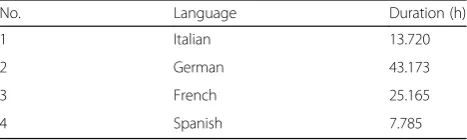
We evaluate and train our end-to-end models on TIMIT dataset, and we use several language resources of Vox-forge dataset to do multilingual training. The augment-ing resources we use are listed in Table1.
All of our end-to-end models are trained with 48 nemes, and there predictions are converted to 39 pho-nemes for scoring. All SA sentences are removed. We followed the common setup of TIMIT. Four hundred sixty-two speakers are selected for train set, 50 speakers are selected for dev set, and 24 speakers are selected for core test set. Durations of them are listed in Table2.
We first train a CTC and an attention-based model separately. Forty mel-scale filterbank coefficients and
Table 1Information of Voxforge multilingual resources
No. Language Duration (h)
1 Italian 13.720
2 German 43.173
3 French 25.165
their delta and delta-delta features are concatenated as their input features.
The baseline CTC model is a five-layer BLSTM with 256 cells in each layer and direction. Dropout rate of 0.2 and 0.5 are applied on inputs and BLSTM separately. For the attention-based model, the encoder is a four-layer BLSTM with 256 cells in each layer and direc-tion. The attention layer is location-based and has 160 cells. The decoder is a one-layer LSTM with 256 cells. Dropout rates for the inputs, the encoder, the attention layer, and the decoder are 0.2, 0.5, 0.1, and 0.1 respect-ively. The optimizer is Adam [25] for both models.
For all end-to-end models, gradient clipping [26] is used for all end-to-end training, and the gradient norm threshold to clip is set to be 5.0. Also, the batch sizes during training are all set to be 32.
4.2 Evaluation measurement
Phone error rate (PER) is adopted to measure the per-formance of speech recognition systems. This score is calculated with the following equation:
PER¼nInsþnDelþnSub
N 100% ð20Þ
wherenIns,nDel, andnSub are number of insert errors, delete errors, and substitute errors, respectively.Nis the total number of phones in the ground truth labels.
4.3 Transfer learning based experiments
We then evaluate on our proposed methods. Firstly, a joint CTC-attention model is trained with the same fil-terbank features. We compare two structures according to our experience. For CTC4 + att4, the CTC part is a four-layer BLSTM with 256 cells and the attention-model has a four-layer BLSTM encoder with 256 cells in each layer and direction, an attention layer with 128 cells, and a one-layer LSTM decoder with 256 cells. The CTC5 + att4 only has more layers of BLSTM for the CTC part, and the rests are the same. For the rest of the joint models in our experiments, they are named by the same manner. For all joint end-to-end models, we set most of the configurations to be the same. The optimizer is AdaDelta [27] function with a learning rate of 10–3. Dropout rate of 0.2 is applied to all BLSTM layers. The MTL weight and the decoding weight for CTC are both 0.3. The width for beam research in de-coding stage is 20. The model which has the best
accuracy evaluated by dev set is chosen to be the final model after 30 epochs of training.
We then experiment with our multilingual methods. We note that TIMIT is evaluated by phones instead of characters. Therefore, each pronunciation dictionary of Voxforge resources is generated using G2P toolkit [28] respectively under the help of CMU dictionary [29]. This allows DNNs to capture enough acoustic similarities.
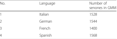
To train multilingual DNNs, we first build their own GMMs. Each GMM is trained using linear discriminative analysis (LDA), maximum linear logistic transformation (MLLT), and speaker adaptive training (SAT) with 13 MFCC features. Then multilingual DNNs are trained with 40 filterbank features of four Voxforge languages simultaneously and are all supervised by alignments of senones generated by each GMM. Numbers of senones for four languages are listed in Table3.
We train our end-to-end models with two types of high-level features as described in Section 2, 4langA-daptBN and 4langAdaptCNMF. For the 4langA4langA-daptBN system, a multilingual bottleneck DNN is trained by four language resources in Voxforge dataset. Each hidden layer has 1026 units (342 units after max pooling) and the bottleneck layer has 120 units (40 units after max pooling). For the 4langAdaptCNMF system, a multilin-gual DNN without bottleneck layers is trained with 1026 units (342 units after max pooling) in each hidden layer.
All DNNs are trained with a dropout rate of 0.2 for other hidden layers. All maxout groups have a pooling size of 3. The Initial learning rate is kept 0.2 for the first 8 epochs and after which is decayed by half when valid-ation error does not decline. The training stops when the validation error finally increases.
For the next step, all parameters below the last shared hidden layer of the multilingual DNN are transferred to a new DNN which is then also re-trained by TIMIT (For the bottleneck multilingual DNN, all parameters below shared bottleneck layer are transferred to a new bottle-neck DNN which is then also re-trained by TIMIT). For the bottleneck features, they are extracted from the re-trained bottleneck layer by feed forward inputs. For the CNMF-based features, we follow exactly the same settings in [20] in our experiments since the approach is sensible to layers and dimensions accorded from the
Table 2Durations of TIMIT dataset
Set Duration (h)
train 3.145
dev 0.342
test 0.162
Table 3Numbers of senones for four languages
No. Language Number of
senones in GMM
1 Italian 1528
2 German 1544
3 French 1400
experience of our prior work. CNMF is applied on the weight matrix from the second last hidden layer, and the dimension for factorization is 40 with 5000 iterations of training. The CNMF-based features are extracted follow-ing the steps described in Section2.
Our high-level features are then sent into joint CTC-attention models for end-to-end training. Unlike a baseline setup, only shallow RNN networks are built for the models. Here we experiment on two structures, namely CTC2 + att2 and CTC3 + att2. We also adjust configurations for these shallow joint models in order to achieve the best performances. Besides different types of input features and number of layers, BLSTM and LSTM are both set to have 320 cells for each layer and direc-tion, and the location-based attention layer has 160 cells.
4.4 Results and discussions
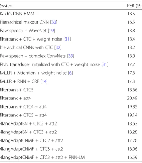
Table 4 shows PERs of all referenced methods and our methods on TIMIT core test set. Below the first line, the first block and the second block shows performances of referenced traditional systems and end-to-end systems respectively. The performances of our results are sum-marized in the last block. We can see that performances of our baseline systems (filterbank + CTC, filterbank + att) cannot compare with referenced methods which use transformed features such as fMLLRs and complex net-works. This is much due to the fact that TIMIT provides a limited resource condition in which purely data-driven training could not satisfied.
For baseline systems, the joint models (filterbank + CTC4 + att4, filterbank + CTC5 + att4) perform better than baseline systems. This demonstrates that joint training and decoder benefits for end-to-end models. We can also conclude from results of filterbank-based systems (filterbank + CTC4 + att4, filterbank + CTC5 + att4), bottleneck-based systems (4langAdaptBN + CTC2 + att2, 4langAdaptBN + CTC3 + att2), and NMF-based systems (4langAdaptCNMF + CTC2 + att2, 4langA-daptCNMF + CTC3 + att2) that a joint model perform better when CTC has one more BLSTM layer than en-coder of attention-based model.
However, performances of filterbank-based systems are still inferior to listed methods due to the lack of trans-formations and regularizations under limited resource condition. The fact that the filterbank-based joint models even perform worse than the CTC baseline sys-tem demonstrates that joint modeling is not enough for solving problem with limited resource.
When multilingual pre-trained bottleneck features are brought in, our systems (4langAdaptBN + CTC2 + att2, 4langAdaptBN + CTC3 + att2) achieve 18.63% and 18.28% on PERs which are comparable to some refer-enced results but are still no better than best end-to-end results. We believe that the disadvantage of setting a bottleneck layer which is analyzed in Section 2 is re-sponsible for this.
When using CNMF to extract features, our best sys-tem (4langAdaptCNMF + CTC3 + att2) obtains a PER of 16.96%. This is superior to all published end-to-end methods in Table 4. Also the fact that NMF approach performs better than bottleneck approach supports our hypothesis (in Section 2.1) that the existence of bottle-neck layers degrades the classification accuracies and could not fully exploit deep transformation of the pre-trained network. These results also strongly support the effectiveness of our CNMF-based approach in end-to-end models.
Although our transfer learning approach requires extra training procedures to extract features, it performs bet-ter with less RNN layers for the end-to-end part.
We also list PERs of some representative traditional methods and notice that published end-to-end models could not beat traditional speech recognition systems. To further compare with the best traditional system which has a language model (LM), we add a small RNN-LM to decode jointly following the method in [18]. The RNN is a two-layer LSTM with 256 cells in each layer and is trained using all transcriptions from the TIMIT train set with a batch size of 32. The LM weight for decoding is 0.2. The result in the last line of Table 4 shows that PER further decreased to 16.59%, which is not only the best among all listed end-to-end results but also is comparable to the state-of-the-art
Table 4PERs of different speech recognition systems on TIMIT core set
System PER (%)
Kaldi’s DNN-HMM 18.5
Hierarchical maxout CNN [30] 16.5
Raw speech + WaveNet [19] 18.8
filterbank + CTC + weight noise [31] 18.4
hierarchical CNNs with CTC [32] 18.2
Raw speech + complex ConvNets [33] 18.0
RNN transducer initialized with CTC + weight noise [31] 17.7
fMLLR + Attention + weight noise [6] 17.6
fMLLR + RNN + CRF [14] 17.3
filterbank + CTC5 18.66
filterbank + att4 20.49
filterbank + CTC4 + att4 19.85
filterbank + CTC5 + att4 19.14
4langAdaptBN + CTC2 + att2 18.63
4langAdaptBN + CTC3 + att2 18.28
4langAdaptCNMF + CTC2 + att2 17.70
4langAdaptCNMF + CTC3 + att2 16.96
performance in TIMIT. Note that our end-to-end models are trained without any regularization except for dropout on BLSTM layers. We believe that our models would benefit more if they were trained with designed regularizations and bigger RNN-LM.
5 Conclusions
A novel transfer learning-based approach is proposed for end-to-end speech recognition. For the first stage, NMF together with multilingual training are used to ex-tract high-level features. For the second stage, joint CTC-attention models are trained on top of the high-level features. Transfer learning is applied through multilingual training and multi-task learning in two levels. Experiments on TIMIT show that our model per-forms the best among all end-to-end models and achieves an extremely close performance compared with the state-of-the-art speech recognition system.
Although our transfer learning approach improves per-formances of end-to-end speech recognition models in TIMIT, it needs to be tested whether this approach also works for relatively high-resource (more than thousands of hour’s data) end-to-end training. What is more is this approach remains a two-stage training fashion which is not a standard end-to-end way. Therefore optimizing fea-ture extraction and RNN training with only one objective function is another job to do. This would require proper tasks separation and intermediate supervisions.
Funding
This work was supported in part by the National Natural Science Foundation of China (No. 61673395, and No. 61403415), Natural Science Foundation of Henan Province (No. 162300410331).
Authors’contributions
C-XQ and DQ conceived and designed the study. C-XQ performed the exper-iments. C-XQ and DQ wrote the paper. C-XQ, DQ, and L-HZ reviewed and edited the manuscript. All authors read and approved the manuscript.
Authors’information
Chu-Xiong Qin was born in Shijiazhuang, China, in 1991. He received the B.S. and M.S. degrees in information and communication from the National Digital Switching System Engineering and Technological R&D Center, Zhengzhou, China, in 2013 and 2016, respectively. He is currently working towards the Ph.D. degree on speech recognition at the National Digital Switching System Engineering and Technological R&D Center. His research interests are in speech signal processing, continuous speech recognition, and machine learning. Dan Qu received the M.S. degree in communication and information system from Xi’an Information Science and Technology Institute, Xi’an, China, in 2000 and the Ph.D. degree in information and communication engineering from the National Digital Switching System Engineering and Technological R&D Center, Zhengzhou, China, in 2005. She is an Associate Professor at the National Digital Switching System Engineering and Technological R&D Center. Her research interests are in speech signal processing and pattern recognition. Lian-Hai Zhang received the M.S. degree in information and communication engineering from the National Digital Switching System Engineering and Technological R&D Center, Zhengzhou, China, in 2000. He is an Associate Professor at the National Digital Switching System Engineering and Technological R&D Center. His research interests are in speech signal processing.
Competing interests
The authors declare that they have no competing interests.
Publisher’s Note
Springer Nature remains neutral with regard to jurisdictional claims in published maps and institutional affiliations.
Author details
1
National Digital Switching System Engineering and Technological R&D Center, Zhengzhou, China.2The State Key Laboratory of Integrated Services Networks, Xidian University, Xi’an, China.
Received: 29 July 2018 Accepted: 28 September 2018
References
1. Graves, A., & Gomez, F. (2006). Connectionist temporal classification: Labelling unsegmented sequence data with recurrent neural networks. In
International Conference on Machine learning (ICML)(pp. 369–376). 2. Chorowski, J., Bahdanau, D., Cho, K., & Bengio, Y. (2014). End-to-end
continuous speech recognition using attention-based recurrent NN: First results.arXiv preprint arXiv, v1412, 1602.
3. Graves, A., & Jaitly, N. (2014). Towards end-to-end speech recognition with recurrent neural networks. InInternational Conference on Machine Learning (ICML)(pp. 1764–1772).
4. D. Amodei, R. Anubhai, E. Battenberg,et al,“Deep speech 2: End-to-end speech recognition in English and mandarin,”Computer Science, 2015. 5. Panayotov, V., Chen, G., Povey, D., & Khudanpur, S. (2015). Librispeech: An
ASR corpus based on public domain audio books. InIEEE International Conference on Acoustics, Speech and Signal Processing (ICASSP). 6. Chorowski, J. K., Bahdanau, D., Serdyuk, D., Cho, K., & Bengio, Y. (2015).
Attention-based models for speech recognition. InAdvances in Neural Information Processing Systems (NIPS)(pp. 577–585).
7. Vaněk, J., Zelinka, J., Soutner, D., & Psutka, J. (2017). A regularization post layer: An additional way how to make deep neural networks robust. InInternational Conference on Statistical Language and Speech Processing (ICASSP).
8. Hannun, A., Case, C., Casper, J., et al. (2014). Deep speech: Scaling up end-to-end speech recognition.arXiv preprint arXiv, 1412, 5567.
9. Chan, W., Jaitly, N., Le, Q., & Vinyals, O. (2016). Listen, attend and spell: A neural network for large vocabulary conversational speech recognition. In
IEEE International Conference on Acoustics, Speech and Signal Processing (ICASSP)(pp. 4960–4964).
10. Chiu, C. C., Sainath, T. N., Wu, Y., Prabhavalkar, R., Nguyen, P., Chen, Z., Kannan, A., Weiss, R. J., Rao, K., Gonina, K., et al. (2018). State-of-the-art speech recognition with sequence-to-sequence models.arXiv preprint arXiv, 1712, 01769.
11. Zhang, Y., Chan, W., & Jaitly, N. (2017). Very deep convolutional networks for end-to-end speech recognition. InIEEE International Conference on Acoustics, Speech and Signal Processing (ICASSP).
12. Sercu, T., & Goel, V. (2016). Dense prediction on sequences with time-dilated convolutions for speech recognition.arXiv preprint arXiv, 1611, 09288. 13. Wang, Y., Deng, X., Pu, S., & Huang, Z. (2017). Residual convolutional CTC
networks for automatic speech recognition.arXiv preprint arXiv, 1702, 07793. 14. Lu, L., Kong, L., Dyer, C., & Smith, N. A. (2017). Multi-task learning with CTC
and segmental CRF for speech recognition.arXiv preprint arXiv, 1702, 06378. 15. Kim, S., Hori, T., & Watanabe, S. (2017). Joint CTC-attention based end-to-end
speech recognition using multi-task learning. InIEEE International Conference on Acoustics, Speech and Signal Processing (ICASSP).
16. Huang, J. T., Li, J., Yu, D., Deng, L., Gong, Y., et al. (2013). Cross-language knowledge transfer using multilingual deep neural network with shared hidden layers. InIEEE International Conference on Acoustics, Speech and Signal Processing (ICASSP).
17. Deng, J., Xia, R., Zhang, Z., Liu, Y., & Schuller, B. (2014). Introducing shared-hidden-layer autoencoders for transfer learning and their application in acoustic emotion recognition. InIEEE International Conference on Acoustics, Speech and Signal Processing (ICASSP).
19. Van Den Oord, A., Dieleman, S., Zen, H., et al. (2016). Wavenet: A generative model for raw audio.arXiv preprint arXiv, 1609, 03499.
20. Qin, C., & Zhang, L. (2016). Deep neural network based feature extraction using convex-nonnegative matrix factorization for low-resource speech recognition. InInformation Technology, Networking, Electronic and Automation Control Conference (ITNEC).
21. Wall, M. E., Rechtsteiner, A., & Rocha, L. M. (2003). Singular value
decomposition and principal component analysis. InA practical approach to microarray data analysis(pp. 91–109). Boston, MA: Springer.
22. Xue, J., Li, J., & Gong, Y. (2013). Restructuring of deep neural network acoustic models with singular value decomposition. InInterspeech(pp. 2365–2369).
23. Ding, C. H., Li, T., & Jordan, M. I. (2010). Convex and semi-nonnegative matrix factorizations.IEEE transactions on pattern analysis and machine intelligence, 32(1), 45–55.
24. T. Hori, S. Watanabe, and J. Hershey,“Joint CTC/attention decoding for end-to-end speech recognition,”Proceedings of the 55th Annual Meeting of the Association for Computational Linguistics. Vol. 1. 2017.
25. Kingma, D. P., & Ba, J. (2014). Adam: A method for stochastic optimization.
arXiv preprint arXiv, 1412, 6980.
26. Pascanu, R., Mikolov, T., & Bengio, Y. (2012). On the difficulty of training recurrent neural networks.arXiv preprint arXiv, 1211, 5063.
27. Zeiler, M. D. (2012). Adadelta: an adaptive learning rate method.arXiv preprint arXiv, 1212, 5701.
28. Bisani, M., & Ney, H. (2008). Joint-sequence models for grapheme-to-phoneme conversion.Speech Comm., 50(5), 434–451.
29. R. L. Weide,“The CMU pronouncing dictionary,”URL:http://www.speech.cs. cmu.edu/cgi-bin/cmudict, 1998.
30. Tóth, L. (2015). Phone recognition with hierarchical convolutional deep maxout networks.EURASIP Journal on Audio, Speech, and Music Processing, vol. 2015, no. 1, pp. 1–13.
31. Graves, A., Mohamed, A. R., & Hinton, G. (2013). Speech recognition with deep recurrent neural networks. InIEEE International Conference on Acoustics, Speech and Signal Processing (ICASSP)(pp. 6645–6649). 32. Zhang, Y., Pezeshki, M., Brakel, P., Zhang, S., Bengio, C. L. Y., & Courville, A.
(2017). Towards end-to-end speech recognition with deep convolutional neural networks.arXiv preprint arXiv, 1701, 02720.