Interpretable Predictive Modeling for Climate Variables with Weighted Lasso

(1)

The Thirty-Third AAAI Conference on Artificial Intelligence (AAAI-19)

Interpretable Predictive Modeling for Climate Variables with Weighted Lasso

Sijie He,

1

Xinyan Li,

1

Vidyashankar Sivakumar,

1

Arindam Banerjee

1 1_{Depertment of Computer Science & Engineering}

University of Minnesota, Twin Cities Minneapolis, MN 55455

[email protected], [email protected], [email protected], [email protected]

Abstract

An important family of problems in climate science focus on finding predictive relationships between various climate variables. In this paper, we consider the problem of predict-ing monthly deseasonalized land temperature at different lo-cations worldwide based on sea surface temperature (SST). Contrary to popular belief on the trade-off between (a) sim-ple interpretable but inaccurate models and (b) comsim-plex ac-curate but uninterpretable models, we introduce a weighted Lasso model for the problem which yields interpretable re-sults while being highly accurate. Covariate weights in the regularization of weighted Lasso are pre-determined, and proportional to the spatial distance of the covariate (sea sur-face location) from the target (land location). We establish fi-nite sample estimation error bounds for weighted Lasso, and illustrate its superior empirical performance and interpretabil-ity over complex models such as deep neural networks (Deep nets) and gradient boosted trees (GBT). We also present a de-tailed empirical analysis of what went wrong with Deep nets here, which may serve as a helpful guideline for application of Deep nets to small sample scientific problems.

Introduction

Over the past decade climate datasets with improved spa-tial resolutions have become available. While such datasets come from a mix of real observations and physics based models, recent years have seen considerable interest in ap-plying machine learning techniques for predictive modeling of climate variables of interest. Such models have the po-tential to aid a better understanding of the impact of climate change and attribution of observed events as well as guide decision/policy making in a variety of domains such as agri-cultural planning, water resource management, and extreme weather events (O’Brien et al. 2006).

We consider one such problem in climate science of identifying predictive relationships between ocean sea sur-face temperature (SST) and land temperature (Steinhaeuser, Chawla, and Ganguly 2011a). Recent work has shown sparse modeling techniques like Lasso (Chatterjee et al. 2012) tend to better capture predictive relationships between SST and land climate compared to more traditional meth-ods like principal component regression (PCR) (Francis

(2)

regularization type, etc. The key factor limiting the perfor-mance is sample size. Deep nets overfit the training set lead-ing to poor validation/test performance. The results empha-size the need for caution and further work on Deep nets for small sample (scientific) problems.

Our main contributions in this paper are as follows: 1. We suggest the weighted Lasso estimator, which

incorpo-rates domain knowledge for finding relationships in spa-tial data. We also derive non-asymptotic parameter esti-mation error bounds for the weighted Lasso estimator. 2. We show that weighted Lasso achieves high prediction

ac-curacy and consistent variable selection for land climate prediction using SST compared to other latest state-of-the-art machine learning methods like Deep nets and gra-dient boosted trees.

3. We perform extensive experiments with Deep nets and show that Deep nets easily overfit the training data with-out sufficient samples.

Organization of the paper: We start with a discussion on related work. We then give finite sample estimation error bounds for weighted Lasso. We subsequently present exper-imental results comparing the weighted Lasso with baseline methods along with in-depth results on Deep nets.

Related work

We briefly review the statistical models used in the climate sciences to discover predictive relationships between cli-mate variables. Most statistical models perform some form of dimensionality reduction due to the large spatial datasets and relatively fewer data samples. A popular method is prin-cipal component regression (PCR) (Olivieri 2018), which has been used for temperature and precipitation prediction in New Zealand (Francis and Renwick 1998). In (Hsieh and Tang 1998), principal component analysis (PCA) is used to compress large spatial fields followed by fitting a neural net-work on the compressed dataset. In (Steinhaeuser, Chawla, and Ganguly 2011a) clustering is used for dimension reduc-tion followed by various regression methods, such as lin-ear regression, support vector regression, regression trees, to predict land temperature and precipitation from global SST field. In contrast (Chatterjee et al. 2012) model the same problem in (Steinhaeuser, Chawla, and Ganguly 2011a) as a high-dimensional sparse regression problem where the land climate is the dependent variable, SST field are the inde-pendent variables and a sparsity promoting regularizer cap-tures the constraint that land temperature is influenced by only a few ocean locations. More recently a spectral nonlin-ear dimensionality reduction method is used in (DelSole and Banerjee 2017) to capture the relationship between summer Texas area temperature and Pacific SST.

Geostatistical methods, like kriging (Goovaerts 1999) and its variations have been applied for spatial interpolation of climate variables (Aalto et al. 2013). However, such meth-ods usually only perform well within a defined local neigh-borhood (Walter et al. 2001). Morevover the success of such methods relies on proper choice of kernels and hyperparam-eters which is statistically and computationally challenging in high-dimensional datasets.

There is increasing interest in exploring the application of Deep nets in climate applications inspired by their success in domains like image processing (He et al. 2016), speech recognition (LeCun, Bengio, and Hinton 2015), etc. Recent work explore the use of Deep nets for prediction of the Oceanic Ni˜no Index (ONI) (McDermott and Wikle 2017) and for statistical downscaling of climate variables (Vandal et al. 2017), although there is currently lacking an under-standing or comprehensive study on the generalization per-formance of Deep nets on small sample size datasets rou-tinely found in climate science applications.

Estimation Error Bound for Weighted Lasso

For land climate prediction using SST, the spatial informa-tion can be considered while designing the predictive mod-els. Since land temperature is known to be mostly influenced by nearby ocean locations, we propose a modification of the weightedℓ1regularizer used in weighted Lasso. It penalizes differently for temperature at each ocean location based on their distance from land target region.

In this section, we provide the non-asymptotic estimation error bound for the following weighted Lasso estimator in a general setting,

ˆ

θ= argmin θ∈Rp

1

2n∥y−Xθ∥ 2

2+λ

p ∑

i=1

wi|θi| (1)

where, for our application,y ∈_Rn_{is the land temperature,} X ∈ Rn×p are SST at pocean locations,θ ∈ Rp are re-gression coefficients,θi is theith coefficient inθ,wiis the positive weight corresponding toθi, andλis penalty param-eter. The weights can be assigned in a data-dependent way or chosen intelligently using prior knowledge. For example, in our application, the weightswi, 1 ≤i≤pare assigned to be proportional to the distance of the ocean location from the land location.

The weighted Lasso estimator is equivalent to the adap-tive Lasso estimator (Zou 2006), except for the procedure used to define the weightswi, 1≤i≤p. While prior work has focused on analysis of the adaptive Lasso estimator in the asymptotic setting (Zou 2006; Huang, Ma, and Zhang 2008), we derive results for the weighted Lasso estimator in the non-asymptotic setting. The results can also be suitably extended to the adaptive Lasso estimator.

Assumptions:Consider data generated according to the lin-ear modelyi=⟨xi, θ∗⟩+ϵi, 1≤i≤nandθ∗is estimated using the weighted Lasso estimator. The rows of the design matrix X ∈ Rn×p are independent sub-Gaussian random vectors with sub-Gaussian norm bounded byLand covari-ance matrixΣ =E[xixTi]. The noiseϵi∈R, 1 ≤i≤nis mean-zero i.i.d. sub-gaussian noise with sub-Gaussian norm less than 1. Assume the following,

1. The true parameter θ∗ is s-sparse. Let w↑ denote the weight vector with elements in ascending order. We assume that the weights corresponding to thesnon-zero elements in θ∗are among the smallestmweightsw↑_1:_minw. Also, let ˆ

(3)

Table 1: Description of the Earth System Models used in the experiments.

Model name Origin Reference

CMCC-CESM Centro Euro-Mediterraneo per I Cambiamenti Climatici (Italy) (Fogli et al. 2009) INM-CM4 Institute for Numerical Mathematics (Russia) (Volodin, Dianskii, and Gusev 2010)

MIROC5-r1i1p1

Atmosphere and Ocean Research Institute, National Institute for Environmental Studies, Japan Agency for Marine-Earth Science and Technology,

University of Tokyo (Japan)

(Watanabe et al. 2010)

M⊥_{is the orthogonal subspace.} 2. When penalty parameterλsatisfies

λ≥c′∗max

{ √ m

√

n∥w_1:↑_m∥2 ,

√

logp

√

nw˜min }

, (2)

wherec′>0is a constant,andw˜minis the minimum element inM⊥_(w↑₎_{, the error set is}

Er={∆∈Rp|R(M⊥(∆))≤β∥w↑1:m∥2∥M(∆)∥2}, (3) whereβ >1is a constant andR(θ) =∑p_i₌₁wi|θi|. The re-stricted eigenvalue (RE) condition (Bickel, Ritov, and Tsy-bakov 2009) is assumed to be satisfied.

Theorem 1. Under the above assumptions, the following bound holds on the error vector∆ = ˆθ−θ∗with high prob-ability for some positive constantc,

∥∆∥2≤ c

√

n (

√

m+∥w ↑ 1:m∥2

√

logp ˜

wmin )

. (4)

Remark 1. For Lassowi = 1, 1 ≤ i ≤ p. Hence in the

context of the above result we recover the non-asymptotic estimation error of Lasso (Chandrasekaran et al. 2012; Negahban et al. 2012; Bickel, Ritov, and Tsybakov 2009) by substitutingm=s,∥w_1:↑_m∥2=

√

sandw˜min= 1.

Remark 2. If the s lowest weights in w↑ _{correspond to} the non-zero weights inθ∗ then we note thatm = sand ∥w_1:↑_s∥2/wmin˜ ≤ √sthus giving an improvement over the corresponding bound for Lasso.

Remark 3. If we end up assigning the largest weights to the non-zero elements inθ∗thenm=pand we recover the bound ∥∆∥2 ≤

√

p/n which is equivalent to performing ordinary least squares on the dataset.

The weighted Lasso problem can be numerically opti-mized by converting it to a Lasso problem by rescaling the data with the weights (Zou 2006).

Land Temperature Prediction

We analyze relationships between land temperature and SST in Earth system model (ESM) data. ESMs are numer-ical models representing physnumer-ical processes in the ocean, cryosphere and land surface with data generated using simu-lations with different initial conditions (Taylor, Stouffer, and Meehl 2012; Pachauri et al. 2014).

We use data from the historical runs of 3 ESMs (see Table 1) included as part of the core set of experiments in CMIP5 (Taylor, Stouffer, and Meehl 2012). The historical runs of CMIP5 ESMs try to replicate observed climate conditions from 1850-2005 closely, capturing effects from changes in atmospheric CO2 due to both anthropogenic and volcanic influences, solar forcing, land use, etc. Each monthly ESM dataset has SST data over a2.5◦×2.5◦ resolution grid of earth and corresponding monthly surface temperature over land locations. In effect for each ESM we have 1872 data points with 5881 ocean locations. Brazil, Peru, and South-east Asia are selected as the 3 land target regions to study in this paper as they are known to have diverse geological properties (Steinhaeuser, Chawla, and Ganguly 2011b).

Experiment Setting

We divide the data into 10 training sets by applying a moving window of 100 years with a stride of 5 years. The 10 years subsequent to the end of the training set are used for testing. We deseasonalize each training-test set combination sepa-rately by z-scoring each month data with the corresponding monthly mean and standard deviation. Note that both train and test sets are z-scored using monthly means and standard deviations computed from the training set. We compare the performance of weighted Lasso against the following base-line methods:

1. ℓ1penalized least squares (Lasso) (Tibshirani 1996): This is equivalent to setting all weights in weighted Lasso equal to1.

2. Principal Component Regression (PCR) (Jolliffe 2011): A popular method in climate science where principal components computed from training data are considered as covariates for ordinary least square regression on re-sponse variables.

3. Gradient Boosted Trees (GBT) (Chen and Guestrin 2016): An ensemble method which uses decision tree as its weak learner. GBTs are implemented in Python using xgboostpackage (Chen and Guestrin 2016).

4. Deep neural networks (Deep nets) (LeCun, Bengio, and Hinton 2015) Multilayer perceptrons with many hid-den layers and CNNs. All networks are implemented in Python usingKeraspackage (Chollet 2015).

(4)

Table 2: Comparison of RMSE on test sets for land climate prediction of Brazil, Peru and South-east Asia using weighted Lasso and other baseline methods. Average RMSE±standard error on test sets are shown. The minimum average RMSE for each target region is shown as bold. Weighted Lasso achieves overall best performance. Furthermore, linear model weighted Lasso and Lasso both outperform Deep nets and GBT.

Model Location Weighted Lasso Lasso PCR Deep nets GBT

CMCC -CESM

Brazil 0.6580±0.0344 0.6681±0.0317 0.8629±0.0654 0.8151±0.0364 0.7354±0.0377 Peru 0.6901±0.0269 0.7120±0.0214 0.8541±0.0560 0.8476±0.0283 0.7400±0.0251 SE Asia 0.5217±0.0103 0.5284±0.0109 0.7252±0.0544 0.7424±0.0153 0.5774±0.0171

INM _-CM4

MIR

OC5

-r1i1p1

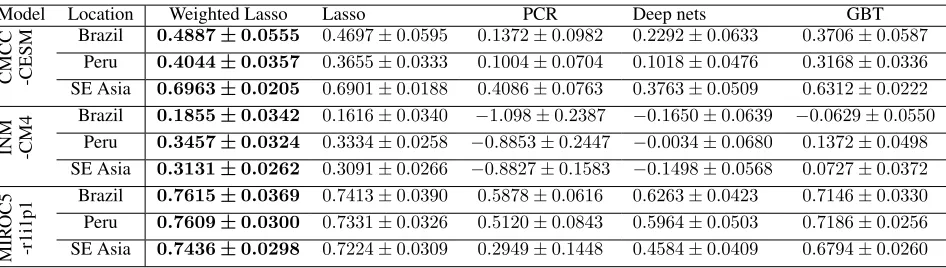
Table 3: Comparison ofR2on test sets for land climate prediction of Brazil, Peru and South-east Asia using weighted Lasso and other baseline methods. AverageR2_±_{standard error on test sets is shown. The maximum average}_R2_{for each target region} is shown as bold. Weighted Lasso achieves overall best predictive performance. Furthermore, linear model weighted Lasso and Lasso both outperform Deep nets and GBT.

Model Location Weighted Lasso Lasso PCR Deep nets GBT

CMCC -CESM

INM _-CM4

Brazil 0.1855±0.0342 0.1616±0.0340 −1.098±0.2387 −0.1650±0.0639 −0.0629±0.0550 Peru 0.3457±0.0324 0.3334±0.0258 −0.8853±0.2447 −0.0034±0.0680 0.1372±0.0498 SE Asia 0.3131±0.0262 0.3091±0.0266 −0.8827±0.1583 −0.1498±0.0568 0.0727±0.0372

MIR

OC5

-r1i1p1

ˆ yi)2/

∑n

i=1(yi −y)¯ 2, where for the i-th data point, yi is the true normalized land temperature for a target region and yˆi is the corresponding estimated value. y¯ is the av-erage value for alln data points. The hyperparameters for weighted Lasso (regularization parameter), Lasso (regular-ization parameter), PCR (number of principal components for regression) and GBT (learning rate and maximum depth of tree) are selected by validation set. Specifically, in each training set we select the first 80 years to train the model and use the next 20 years as a validation set. The hyperpa-rameters giving best performance on the validation set are chosen. We then refit the predictive models on the full train-ing set ustrain-ing the chosen hyperparameters. For GBT, we fix the number of trees to 100, and perform a grid-search to find the optimal learning rate and maximum depth of tree. For all models the optimal value of learning rate on the validation set varies between 0.05 and 0.07 and the optimal maximum tree depth is found to be 3. For Deep nets we experiment with various combinations of: (a) the number of hidden lay-ers, (b) the number of hidden units in each layer, (c) differ-ent mini-batch size when training using the Adam optimiza-tion algorithm (Kingma and Ba 2014), and (d)ℓ1, ℓ2 and

no regularization. Each network uses Relu (Nair and Hin-ton 2010) as activation function. The maximum number of epochs for training is set as 150. We also use early-stopping by examining validation set error. In almost all cases, an 8 hidden layer Deep nets withℓ1regularization on the weights gave the best performance on the validation set. We report results with mini batch size set to 32. We also run experi-ments with transfer learning (Yosinski et al. 2014) for Con-volutional Neural Networks (CNN) (Lecun et al. 1998) by training only the last two layers of the Resnet-50 (He et al. 2016) which is pre-trained on ImageNet (Russakovsky et al. 2015). Resnet-50 is found to have worse performance in comparison to Deep nets and hence, in the interest of brevity and space, we exclude it from the comparison. More details on the performance of Resnet-50 can be found in Table 6.

Experimental Results

(5)

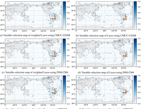
(a) Variable-selection map of weighted Lasso using CMCC-CESM (b) Variable-selection map of Lasso using CMCC-CESM

(c) Variable-selection map of weighted Lasso using INM-CM4 (d) Variable-selection map of Lasso using INM-CM4

(e) Variable-selection map of weighted Lasso using MIROC5 (f) Variable-selection map of Lasso using MIROC5

Figure 1: Comparison of variable selection by Lasso and weighted Lasso for Brazil temperature prediction. The plot shows the probability that each ocean location is selected in the 10 runs for each ESM model. In contrast to Lasso, weighted Lasso chooses more ocean locations closer to Brazil and achieves more consistent variable selection.

Prediction AccuracyTable 2 and Table 3 report the aver-age RMSE,R2, and their standard errors. Weighted Lasso achieves better average predictive accuracy compared to other baseline methods across all 3 ESMs. The p-values of 2-sample K-S test (Daniel 1978) for RMSE on test sets are shown in Table 4. Weighted Lasso is significantly better than PCR, Deep nets and GBT (p <0.05) in most cases (21 out of 27). While the prediction accuracy of weighted Lasso is not significantly better than Lasso, we show that weighted Lasso consistently chooses a subset of variables of which ocean locations are close to the land target region, which is more interpretable in climate science perspective.

Variable selection Weighted Lasso and Lasso introduce sparsity in variable selection. During the training phase, an ocean location is considered selected, if it has a correspond-ing non-zero coefficients. The behavior of weighted Lasso (and Lasso respectively) is similar for land climate predic-tion across 3 land target regions. We analyze the ocean loca-tions selected by Lasso and weighted Lasso for Brazil

(6)

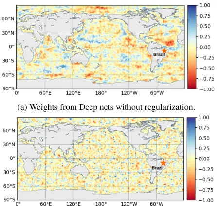
(a) Weights from Deep nets without regularization.

(b) Weights from Deep nets withℓ1regularization.

Figure 2: Comparison of regression coefficients of a unit from Deep nets with and withoutℓ1regularization for Brazil. All weights are normalized to[−1,1]by dividing the largest value among absolute weights.

Deep nets: What happened?

In this section, we analyze various facets of the performance of Deep nets. The performance of Deep nets is influenced by the number of hidden layers, number of hidden units, mini-batch size, regularization etc. We analyze the impact of each of these on the performance of Deep nets by vary-ing one of the parameters while keepvary-ing the others fixed. We also demonstrate that Deep nets overfit the training data and hence do not generalize well on the test set.

Overfitting Figure 3 shows the training and validation set RMSE after each epoch for a 8 layer Deep nets with 32 hid-den units trained for temperature prediction over Brazil. The

Table 4: The p-values from 2-sample KS-test on RMSE of test sets of weighted Lasso against other baseline methods are shown. The p-values less than 0.05 are shown in bold. The performance of weighted Lasso is significantly better than non-linear baseline methods for most of target regions.

Model Location Lasso PCR Deep nets GBT

CMCC -CESM

Brazil 0.9747 0.1108 0.0310 0.1108 Peru 0.6750 0.3128 0.0068 0.3128 SE Asia 0.6750 0.0001 0.0000 0.0068

INM _-CM4

MIR

OC5

-r1i1p1

Figure 3: An example of model overfitting during the train-ing phase for Deep nets. Deep nets are trained for 150 epochs. The blue curve and orange curve indicate the RMSE of the training and validation set for Deep nets. There is a clear gap between the training and validation RMSE. The RMSE of weighted Lasso on both training (green line) and validation (red line) sets are also shown for comparison.

Deep nets training error stabilizes after about 20 epochs and is lower than the RMSE of linear models. In contrast the validation set error of the Deep nets is much higher which indicates that Deep nets overfit the noise in the training set and hence can not generalize well over the unseen test set. Effect of number of hidden units Figure 4 plots the test RMSEs for temperature prediction over Brazil as we alter the number of hidden units in each layer. The RMSE slightly decreases as the number of hidden units increases from 1 to 64 for both shallow networks with 1 hidden layer, and Deep nets with 8 hidden layers.

(7)

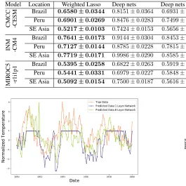
Table 5: Comparison of RMSE on test sets of regularized Deep nets and weighted Lasso. Average test RMSE±standard error are shown. Deep nets withℓ1regularization has smaller test set RMSE thanℓ2andℓ1+ℓ2regularization.

Model Location Weighted Lasso Deep nets Deep nets withℓ1 Deep nets withℓ2 Deep nets withℓ1+ℓ2

CMCC -CESM

INM _-CM4

MIR

OC5

-r1i1p1

Figure 5: The comparison of predicted land temperatures in Brazil with CMCC-CESM over a 10 year period (1950-1960) between a shallow and a deep network structure. The deep structure predictions are better than a shallow network.

Table 6: Comparison of the best RMSEs among weighted Lasso, Deep nets, and Resnet-50 using data from CMCC-CESM. Resnet-50 shows worse predictive accuracy com-pared to other methods.

Location Weighted Lasso Deep nets Resnet-50 Brazil 0.6513±0.0635 0.8151±0.0364 1.2972±0.4109

Peru 0.6944±0.0444 0.8476±0.0283 1.3739±0.3211

SE Asia 0.5162±0.0213 0.7424±0.0153 1.4760±0.4227

Effect of mini-batch sizeMini-batch size while training is believed to have a strong impact on Deep nets performance (Bengio 2012; Masters and Luschi 2018). We analyze the effect on average test RMSE of mini-batch size for temper-ature prediction over all three land locations (Figure 6). The RMSE are highest with small batch sizes, steadily decreas-ing with increasdecreas-ing batch size.

Effect of Regularization We explore 3 regularization schemes, ℓ1, ℓ2 and ℓ1 +ℓ2. Table 5 shows the compari-son on the test RMSE values of weighted Lasso and Deep nets before and after applyingℓ1, andℓ2regularization.ℓ1 regularization seems to give better performance over other regularization schemes including no regularization.

Conclusions

In this paper, we propose a weighted Lasso scheme for pre-diction on spatial climate data in order to encode the

in-Figure 6: Average test RMSE vs mini batch size over Brazil, Peru, and SE Asia for ESM model CMCC. Mini batch size of 1, 2, 4, 8, 16, 32, 64, 128, 256, 512 as well as full batch size are used on a 8 hidden layer network. The average RMSE on test sets decreases as batch size increases.

herent spatial information in such datasets. Also, the non-asymptotic estimation error bound for weighted Lasso is given. The proposed method is evaluated on a task to pre-dict temperature for 3 distinct land target regions using SST from the historical runs of 3 ESMs. The weights are set to be proportional to the geographical distance between the ocean location of each predictor and the target land region, con-straining the estimator to pick spatially nearby ocean loca-tions. Weighted Lasso not only achieves better prediction ac-curacy compared to other linear and non-linear models, in-cluding PCR, GBT and Deep nets across all ESMs, but also selects stable predictors consistent with domain knowledge. We also conduct a comprehensive analysis of Deep nets on high-dimensional climate datasets with small sample size. Empirical results show that linear models outperform the non-linear models and thus are more suitable for climate problems where the number of samples is limited.

Acknowledgments

(8)

References

Aalto, J.; Pirinen, P.; Heikkinen, J.; and Ven¨al¨ainen, A. 2013. Spa-tial interpolation of monthly climate data for finland: comparing the performance of kriging and generalized additive models. The-oretical and Applied Climatology112(1-2):99–111.

Bengio, Y. 2012. Practical Recommendations for Gradient-Based Training of Deep Architectures. Berlin, Heidelberg: Springer Berlin Heidelberg. 437–478.

Bickel, P. J.; Ritov, Y.; and Tsybakov, A. B. 2009. Simultaneous analysis of lasso and dantzig selector. The Annals of Statistics,

1705–1732.

Chandrasekaran, V.; Recht, B.; Parrilo, P. A.; and Willsky, A. S. 2012. The convex geometry of linear inverse problems. Founda-tions of Computational mathematics,12(6):805–849.

Chatterjee, S.; Steinhaeuser, K.; Banerjee, A.; Chatterjee, S.; and Ganguly, A. 2012. Sparse group lasso: Consistency and climate applications. InProceedings of the 2012 SIAM International Con-ference on Data Mining (SDM), 47–58.

Chen, T., and Guestrin, C. 2016. Xgboost: A scalable tree boosting system. InProceedings of the 22nd ACM SIGKDD International Conference on Knowledge Discovery and Data Mining (SIGKDD), 785–794.

Chollet, F. 2015. Keras. https://github.com/fchollet/keras. Daniel, W. W. 1978. Applied nonparametric statistics. Houghton Mifflin.

DelSole, T., and Banerjee, A. 2017. Statistical seasonal prediction based on regularized regression. Journal of Climate,30(4):1345– 1361.

Fogli, P. G.; Manzini, E.; Vichi, M.; Alessandri, A.; Patara, L.; Gualdi, S.; Scoccimarro, E.; Masina, S.; and Navarra, A. 2009. Ingv-cmcc carbon (icc): A carbon cycle earth system model.

CMCC Research Paper,61:31.

Francis, R., and Renwick, J. 1998. A regression-based assessment of the predictability of new zealand climate anomalies.Theoretical and Applied Climatology,60(1):21–36.

Goovaerts, P. 1999. Geostatistics in soil science: state-of-the-art and perspectives.Geoderma89(1-2):1–45.

He, K.; Zhang, X.; Ren, S.; and Sun, J. 2016. Deep residual learn-ing for image recognition. InProceedings of the IEEE conference on computer vision and pattern recognition (CVPR), 770–778. Hsieh, W. W., and Tang, B. 1998. Applying neural network models to prediction and data analysis in meteorology and oceanography.

Bulletin of the American Meteorological Society,79(9):1855–1870. Huang, J.; Ma, S.; and Zhang, C.-H. 2008. Adaptive lasso for sparse high-dimensional regression models. Statistica Sinica,

1603–1618.

Jolliffe, I. 2011. Principal component analysis. InInternational encyclopedia of statistical science. Springer. 1094–1096.

Kingma, D. P., and Ba, J. 2014. Adam: A method for stochastic optimization.arXiv preprint arXiv:1412.6980.

Krizhevsky, A.; Sutskever, I.; and Hinton, G. E. 2012. Ima-genet classification with deep convolutional neural networks. In

Advances in neural information processing systems (NIPS), 1097– 1105.

LeCun, Y.; Bengio, Y.; and Hinton, G. 2015. Deep learning. Na-ture,521(7553):436.

Lecun, Y.; Bottou, L.; Bengio, Y.; and Haffner, P. 1998. Gradient-based learning applied to document recognition. Proceedings of the IEEE,86(11):2278–2324.

Masters, D., and Luschi, C. 2018. Revisiting small batch training for deep neural networks.arXiv preprint arXiv:1804.07612. McDermott, P. L., and Wikle, C. K. 2017. Bayesian recurrent neural network models for forecasting and quantifying uncertainty in spatial-temporal data.arXiv preprint arXiv:1711.00636. Nair, V., and Hinton, G. E. 2010. Rectified linear units improve restricted boltzmann machines. InProceedings of the 27th interna-tional conference on machine learning (ICML), 807–814. Negahban, S. N.; Ravikumar, P.; Wainwright, M. J.; and Yu, B. 2012. A unified framework for high-dimensional analysis ofm -estimators with decomposable regularizers. Statistical Science

27(4):538–557.

O’Brien, G.; O’Keefe, P.; Rose, J.; and Wisner, B. 2006. Climate change and disaster management.Disasters30(1):64–80. Olivieri, A. C. 2018. Introduction to Multivariate Calibration: A Practical Approach. Springer.

Pachauri, R. K.; Allen, M. R.; Barros, V. R.; Broome, J.; Cramer, W.; Christ, R.; Church, J. A.; Clarke, L.; Dahe, Q.; Dasgupta, P.; et al. 2014. Climate change 2014: synthesis report. Contribution of Working Groups I, II and III to the fifth assessment report of the Intergovernmental Panel on Climate Change. IPCC.

Russakovsky, O.; Deng, J.; Su, H.; Krause, J.; Satheesh, S.; Ma, S.; Huang, Z.; Karpathy, A.; Khosla, A.; Bernstein, M.; Berg, A. C.; and Fei-Fei, L. 2015. Imagenet large scale visual recognition chal-lenge. International Journal of Computer Vision,115(3):211–252. Steinhaeuser, K.; Chawla, N.; and Ganguly, A. 2011a. Comparing predictive power in climate data: Clustering matters. Advances in Spatial and Temporal Databases,39–55.

Steinhaeuser, K.; Chawla, N. V.; and Ganguly, A. R. 2011b. Com-plex networks as a unified framework for descriptive analysis and predictive modeling in climate science. Statistical Analysis and Data Mining,4(5):497–511.

Taylor, K. E.; Stouffer, R. J.; and Meehl, G. A. 2012. An overview of cmip5 and the experiment design.Bulletin of the American Me-teorological Society,93(4):485–498.

Tibshirani, R. 1996. Regression shrinkage and selection via the lasso.Journal of the Royal Statistical Society,267–288.

Vandal, T.; Kodra, E.; Ganguly, S.; Michaelis, A.; Nemani, R.; and Ganguly, A. R. 2017. Deepsd: Generating high resolution climate change projections through single image super-resolution. In Pro-ceedings of the 23rd ACM SIGKDD International Conference on Knowledge Discovery and Data Mining (SIGKDD), 1663–1672. Volodin, E.; Dianskii, N.; and Gusev, A. 2010. Simulating present-day climate with the inmcm4.0 coupled model of the atmo-spheric and oceanic general circulations.Atmospheric and Oceanic Physics,46(4):414–431.

Walter, C.; McBratney, A. B.; Douaoui, A.; and Minasny, B. 2001. Spatial prediction of topsoil salinity in the chelif valley, algeria, using local ordinary kriging with local variograms versus whole-area variogram.Soil Research39(2):259–272.

Watanabe, M.; Suzuki, T.; Oishi, R.; Komuro, Y.; Watanabe, S.; Emori, S.; Takemura, T.; Chikira, M.; Ogura, T.; Sekiguchi, M.; et al. 2010. Improved climate simulation by miroc5: mean states, variability, and climate sensitivity. Journal of Climate,

23(23):6312–6335.