by
Subramaniam Venkatraman
A thesis
submitted in partial fulfillment
of the requirements for the degree of
Master of Science in Electrical Engineering
Boise State University
DEFENSE COMMITTEE AND FINAL READING APPROVALS
of the thesis submitted by
Subramaniam Venkatraman
Thesis Title: DEGRADATION SPECIFIC OCR
Date of Final Oral Examination: 15 December 2010
The following individuals read and discussed the thesis submitted by student Subramaniam Venkatraman, and they evaluated his presentation and response to questions during the final oral examination. They found that the student passed the final oral examination.
Elisa Barney Smith, Ph.D. Chair, Supervisory Committee
Thad Welch, Ph.D. Member, Supervisory Committee
Tim Andersen, Ph.D. Member, Supervisory Committee
I would like to thank Dr. Barney Smith who encouraged me all along and kept me
focused and motivated. My thesis would not have been possible without her unending
support and mentoring. The help and support she provided me in this journey have been
invaluable to me to attain this goal.
I am lucky to have a very supporting mother, sister-in-law, and my best friend,
philoso-pher, and guide in my elder brother. I would like to thank my friends Hidayatullah Ahsan,
C. J. Stanger, Thanh Tran, Dr. Vishal Saxena, and others who were of immense help and
provided insight in my work. They helped me overcome stress and frustration that I faced
when I was hitting roadblocks and kept me focused and motivated towards my goal. I am
honored and grateful to my committee members Dr. Tim Andersen and Dr. Thad Welch
who provided time and energy to review this thesis.
Optical Character Recognition (OCR) is the mechanical or electronic translation of
scanned images of handwritten, typewritten, or printed text into machine-encoded text.
OCR has many applications, such as enabling a text document in a physical form to be
editable, or enabling computer searching on a computer of a text that was initially in
printed form. OCR engines are widely used to digitize text documents so that they can
be digitally stored for remote access, mainly for websites. This facilitates the availability
of these invaluable resources instantly, no matter the geographical location of the end user.
Huge OCR misclassification errors can occur when an OCR engine is used to digitize a
document that is degraded. The degradation may be due to varied reasons, including aging
of the paper, incomplete printed characters, and blots of ink on the original document. In
this thesis, the degradation due to scanning text documents was considered. To improve
the OCR performance, it is vital to train the classifier on a large training set that has
significant data points similar to the degraded real-life characters. In this thesis, characters
with varying degrees of blurring and binarization thresholds were generated and they were
used to calculate Edge Spread degradation parameters. These parameters were then used to
divide the training data set of the OCR engine into more homogeneous sets. The resulting
classification accuracy by training on these smaller sets was analyzed.
The training data set consisted of 100,000 data points of 300 DPI, 12 point Sans Serif
font lowercase characters ‘c and ‘e’. These characters were generated with random values
of threshold and blur width with random Gaussian noise added. To group the similar
degraded characters together, clustering was performed using the Isodata clustering
calculated on edges in close proximity accounting for interference effects, named MDC,
were estimated to fit the cluster boundaries. These values were then used to divide the
training data and a Bayesian classifier was used for recognition. It was verified that MDC
is slightly better than DC as a division parameter. A choice of either 2 or 3 partitions was
found to be the best choice for dataset division. An experimental way to estimate the best
boundary to divide the data set was determined and tests were conducted that verified it.
Both crisp and fuzzy approaches for classifier training and testing were implemented
and various combinations were tried with the crisp training and fuzzy testing being the best
approach, giving a 98.08% classification rate for the data set divided into 2 partitions and
98.93% classification rate for the data set divided into 3 partitions in comparison to 94.08%
for the classification of the data set with no divisions.
ABSTRACT . . . iv
LIST OF TABLES . . . viii
LIST OF FIGURES . . . ix
1 INTRODUCTION . . . 1
2 TECHNICAL BACKGROUND . . . 8
2.1 Generating Synthetic Scanned Images . . . 10
2.1.1 Basic Scanner Model . . . 11
2.1.2 Edge Spread, Delta C (DC) . . . 13
2.1.3 Stroke Spread, Modified Delta C (MDC) . . . 16
2.2 Clustering . . . 19
2.2.1 Isodata Clustering . . . 20
2.2.2 Fuzzy C-Means Clustering . . . 20
2.3 Classifiers . . . 22
2.3.1 Bayesian Classifier . . . 24
2.3.2 Crisp Training . . . 26
2.3.3 Fuzzy Training . . . 26
2.3.4 Crisp Testing . . . 27
2.3.5 Fuzzy Testing . . . 27
3.1 Dataset . . . 32
3.2 Analysis of Cutoff Selection for the Number of Pixels in Generated Characters 35 3.3 Implementation Details to Validate the Tests . . . 38
3.3.1 Clustering . . . 39
3.3.2 Fitting DC and MDC Boundaries . . . 42
3.3.3 Partitioning and Classification . . . 47
3.4 Decision on Number of Cluster Partitions and Cluster Boundaries . . . 48
3.5 Exhaustive Cluster Classification Accuracy Analysis . . . 48
3.6 Fuzzy vs Crisp Boundaries and the Need for It. . . 53
4 CONCLUSION AND FUTURE WORK . . . 57
4.1 Future Work . . . 60
5 REFERENCES . . . 62
3.1 Classification results for 2 partitions . . . 54
3.2 Classification results for 3 partitions . . . 55
1.1 Ideal, thin and thick characters ‘c’ and ‘e’. . . 3
2.1 This scanner model is used to determine the value of the pixelf[i,j]centered
on each sensor element[10]. . . 12
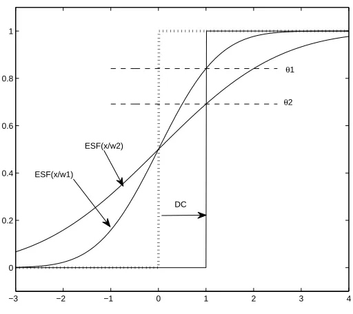
2.2 Gaussian ESFs are shown with w1=1 and w2=2. When the image is blurred
and thresholded, the position of the edge is shifted from the dotted step
function to the solid step edge function. This shift is called DC and is by
convention positive when the edge is shifted to the left [9]. . . 15
2.3 Edge spread degradation parameter DC isocline lines for DC values -0.1,
-0.5, 0, 0.1 and 0.5. . . 16
2.4 When a stroke characterized by two parallel edges is scanned, the resulting
stroke thickness changes. Interference between the parallel edges causes
the grayscale value of pixels to be less than that predicted by the ESF. As a
result, the stroke thickness will be less than that predicted by DC. . . 18
2.5 Edge spread degradation parameter MDC Isocline lines for MDC values
-1.5, -1, 0, 1, and 1.5. . . 19
3.1 (a) Character ‘c’ with noise, (b) filtered image with most of the noise
around the image removed . . . 34
3.2 Characters ‘c’ and ‘e’ are shown with limits of 5, 10, 15, 25, 50, 100, 125
and 150%. . . 37
thresholdθ in degradation space with DC lines drawn, x-axis is PSF width,
y- axis is binarization thresholdθ. . . 40
3.4 2 cluster plot with cutoff on number of black pixels relative to an ideal
character being (a) 100%, (b) 50%, (c) 25%, (d) 15%, (e)10%, (f) 5%. . . 43
3.5 Clustering of character features by width,theta (a) characterc divided into
2 partitions, (b) charactercdivided into 3 partitions, (c) characteredivided
into 2 partitions, (d) characteredivided into 3 partitions, (e) mixed charactesrc
and e divided into 2 partitions,(f) mixed charactesrc ande divided into 3
partitions. . . 44
3.6 2 cluster partitions (a) charactercwith DC = 0.9, (b) charactercwith MDC
= 1, (c) characterewith DC = 0.4, (d) characterewith MDC = 0.6, (e) mixed
charactesrcandewith DC = 0.9,(f) mixed charactesrcandewith MDC = 0.8. 45
3.7 Charactercandemixed dataset (a) divided into 2 partitions and divided by
DC partition, (b) divided into 2 partitions and divided by MDC partition,
(c) divided into 3 partitions and divided by DC partition, (d) divided into 3
partitions and divided by MDC partition. . . 47
3.8 10% thresholded charactercdata (a) divided into 2 partitions, (b) divided
into 3 partitions, (c) divided into 4 partitions, (d)divided into 5 partitions. . . 49
3.9 Accuracy plot, exhaustive division of characters candemixed dataset (a)
by DC for 2 partitions, (b) by MDC for 2 partitions, (c) Samples of ‘c’ and
‘e’ throught the degradation space. DC and MDC lines are shown for the
optimal values for 2 partitions . . . 50
by DC for 3 partitions, (b) by MDC for 3 partitions, (c) samples of ‘c’ and
‘e’ throughout the degradation space. DC and MDC lines are shown for the
optimal values for 3 partitions . . . 52
CHAPTER 1
INTRODUCTION
The world is rapidly moving towards the extensive use of computers and digital media to
access information. An increasing number of people are using the internet as the most
trusted source to get information, search for articles, read the news and update themselves
with all other day to day scholarly as well as routine chores. This transition to digital media
has been made possible by the advancement in internet technology which has kept pace
with this exponential demand and thus we can depend on technology to get information
from remote locations instantaneously. This demand in digital copies has resulted in an
increased demand for journals, articles and other literature to be available in a digitized
version. It is especially useful to have articles that have a limited circulation or availability,
such as old books which are no longer in publication, rare manuscripts and research articles,
available digitally. If we can stay clear of any copyright violation, the digital availability of
these invaluable resources, coupled with the fact that they can be accessed instantly through
the web is invaluable in research and also helps to keep record of previous work. In order to
digitize, it is impractical to get a person to type all these articles, books and other invaluable
literature. This necessitates the use of Optical Character Recognition (OCR) to implement
this conversion from images of text to digital text documents. The OCR engines convert
the undegraded documents into corresponding digital copies with an acceptable accuracy
The documents that are scanned and subsequently converted to digital copies by OCR
engines may be degraded due to various reasons, thus affecting the performance of the
OCR engine. The reasons include improper printing of the original document, aging of the
original book or journal, etc. The degradation effects due to the previously mentioned
reasons are not modeled in this thesis. Degradations introduced due to scanning text
documents are considered in this thesis.
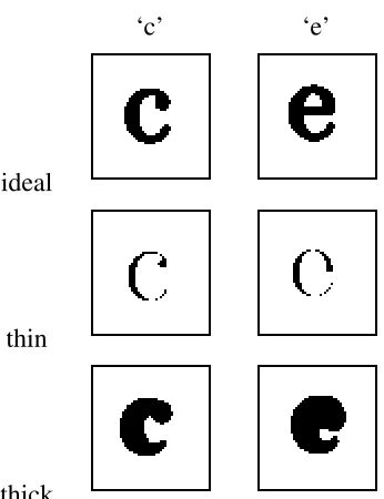
In this thesis, the dataset considered is comprised of characters ‘c’ and ‘e’ because they
pose the biggest challenge for modern day classifiers due to similarities in appearance. If
the classifier performance is good with worst case data, it should perform better on any
other data set. The character appearance variations of printed characters ‘c’ and ‘e’ caused
by scanning degradation with different stroke widths is shown in Figure 1.1. The difference
between the ideal and the degraded character is significant, as seen in the figure. Figure
1.1 shows the ideal printed characters, characters with a thin stroke thickness as well as
characters with thick stroke widths. These variations seen in the character appearance are
due to degradations discussed in detail in the following paragraphs.
We have to make sure that the classifier in the OCR engine is trained on all of the
varia-tions of the characters shown, as these patterns are encountered frequently by OCR engines
in their daily operations. It can be visually concluded that if the OCR engine is trained to
only identify the ideal characters, the non-ideal characters, which are a slight variation of
the ideal characters shown in Figure 1.1, may be misclassified due to insufficient training.
This will lead to a sizeable classification error in the final transcript and hence has to be
handled in training to reduce the error.
‘c’ ‘e’
ideal
thin
thick
Figure 1.1: Ideal, thin and thick characters ‘c’ and ‘e’.
by Baird [10]. When a printed line is scanned, there are two possibilities: thickening or
thinning of the original line. This is referred to as a degradation because the scanned image
is not exactly the same as the original scanned image. Analysis is required to determine
by how much the degradation introduced has thickened or thinned the scanned lines. The
major factors that cause degradation in an image passed through a scanner are the point
spread function (PSF), which causes the blur, and the binarization threshold. The point
spread function describes the effect of reflection of light from the different optics of the
scanner when an image is scanned.
It is relatively common to design classifiers under the assumption that there is large
within class similarity and low between class similarity in the training dataset. The within
class similarity is often increased by restricting the problem to a “common” domain, or
dividing a larger non-homogeneous problem into multiple problems, each of which exhibit
larger homogeneity. This has often been done in OCR problems by assuming a common
a particular font and style requires that some form of font/style detection be employed in
order to select the appropriate classifier (the one that was trained on the font style being
recognized) during execution. To improve classifier performance when the input is not
guaranteed to be homogeneous, it is also desirable to have a large and varied training set
to improve the ability of the classifier to generalize. This, however, leads to lower within
class similarity.
Other approaches have been explored to partition the dataset to improve OCR results.
These vary in the classifier used, training data used, training method employed, and a host
of other factors. The basic idea explored in all the research papers related to this topic is
grouping the training data into isogenous patterns. Xiu et al. [1] talk about a style-based
approach to improve overall accuracy of paper ballot mark recognition to get a valid count
of votes cast in an election. The method used to determine the style did not evaluate every
mark on the ballot in isolation, but the decision was made after analyzing all the marks
made on a particular ballot form by a voter. Thus, the consistency of marks of the voter
across the ballot and the inherent style was used to judge and decide a valid vote. Xiu and
Baird [2] exploited the strong visual consistency of font and degradation within a book,
which is generally an isogenous pattern due to the same font size and font style seen on a
page of text, to conclude the style. The style information was then used as a parameter to
train the classifier and greater accuracy was achieved in the classification of text in books.
Another idea to get more homogeneity within the training dataset is dividing by font
type. Baird and Nagy [3] suggested a way to improve the classification accuracy of a
polyfont classifier that is capable of recognizing any of 100 typefaces moderately well. The
method suggested is to specially train the classifier in the OCR engine on the single font it
is currently analyzing. The decision on the current font and size is arrived at after analyzing
intervention in this otherwise automatic process. Sarkar and Nagy [4, 5, 6] observed that
in many applications of pattern recognition, patterns appear in groups and have a common
origin. An example would be a printed word with characters that comprise that word in
the same font. The common origin leaves its style imprint on its patterns, resulting in style
consistency. Tests were done on handwritten as well as printed text using a style specific
classifier to prove that modeling style dependencies among constituent patterns of a field
improved classification accuracy. This is possible because data used in OCR engines have
different styles that are distinct, and hence this feature has been exploited.
Many approaches have been followed to partition the dataset into smaller homogeneous
partitions to improve the classifier performance. The approach to implement within class
similarity proposed in this thesis is grouping the data by degradation parameters that are
introduced during scanning. This grouping of degraded characters is done based on their
visual appearance (i.e., thick/thin/medium) of the character strokes. The changes in stroke
widths due to scanning have been modeled and a mathematical formula has been developed
to describe them [8, 9]. The model to estimate the stroke thickness uses the blur widthw
and binarization thresholdθ,which in turn relate to edge spread degradation parameters.
Dividing the dataset by the character being thick or thin is one way of partitioning, but there
are numerous other ways that have been explored. Barney Smith and Andersen [7] analyzed
and experimented on how the classifier accuracy of an OCR engine can be improved by
training with a dataset that resembles more closely the degraded character to which the
OCR engine is subjected. They discovered that, while dividing the dataset by width wor
thresholdθ individually improves the performance over classification of an unpartitioned
dataset, the edge spread degradation parameter was a better partitioning parameter
com-pared to others. In spite of all this analysis, there is still room for improvement and we can
be done to come up with answers on how many regions to divide the dataset into, at what
value, what parameter to use, and whether an edge spread model based on isolated edges
or one that considers adjacent edge interference is better.
The tests implemented in this thesis were motivated by the goal to explore and answer
the following six questions. These questions are:
1. Did the division of the dataset improve the accuracy of classifying the dataset?
2. Is an edge spread that considers adjacent edge scanning interference a better
parame-ter to partition the dataset than an edge spread parameparame-ter based on scanning isolated
edges?
3. If the dataset was divided by the incorrect values, how does it affect the performance?
4. What is the reasonable number of partitions into which a dataset should be divided?
5. What is the error associated with estimating the wrong edge spread degradation
parameters for a character?
6. Does the use of a fuzzy approach of classification offer any improvement in
perfor-mance over the crisp approach?
To analyze the ideas suggested in this thesis, many components and algorithms were
im-plemented. Chapter 2 gives technical background related to the division of the dataspace
using edge spread parameters. This chapter includes details of the degradation model that
is used to generate the degraded training set. The edge spread degradation parameters
are introduced and mathematical formulae to estimate them are discussed. This chapter
also describes briefly the Bayesian classifier and the Isodata clustering algorithm used
approaches that have been implemented to improve the performance is presented. Chapter
3 gives details of the experiments done to evaluate how the new edge spread parameter
that considers adjacent edge scanning interference is better than the edge spread parameter
based on scanning of isolated edges. Chapter 4 talks about the analysis and conclusions
that we can arrive at after seeing the results and also a few ideas on further improving the
CHAPTER 2
TECHNICAL BACKGROUND
The dataset used in this thesis is comprised of the degraded characters ‘c’ and ‘e’. These
two characters were selected because of their high visual similarity. These characters pose
the greatest challenge for classifiers to classify and thus are extensively used to evaluate
classifiers. It is very difficult to generate a representative training dataset from scanned
documents. If a training dataset is not a representative dataset, it generally results in a
poorly trained classifier. A scanner model was used to generate synthetic degraded ‘c’
and ‘e’ character samples with varying stroke widths. We generated synthetic characters
instead of real scanned characters because even though we encounter a large variation in
real documents with different stroke widths, calculating the degradation parameters after
these documents are scanned is difficult. This is mainly due to the cost associated with
calibrating real documents, which is time consuming, and thus increases the cost of that
operation. A better, cost effective approach is to synthetically generate characters in the
training dataset with known parameters so that the scanned degradation can be easily
estimated from them. Subsection 2.1.1 will discuss the degradation model used to generate
the degraded characters used to train and evaluate the classifier. Degradation parameters are
calculated from the characters that will then be used to divide the training dataset. In this
thesis, the degradation parameters that are being considered are edge spread degradation
which is applicable to edges in isolation and is a combination of w and θ called DC. It
was initially used to partition the degradation space by Barney Smith and Andersen [7]
and proved to be a better division parameter than using either undivided data, division by
PSF width or binarization threshold alone. McGillivary [9] developed a formulation for the
edge spread when two edges are close enough to interfere called MDC. This parameter is
a better description of the stroke width changes when lines or strokes frequently seen in
real-life text are scanned. Section 2.1.3 elaborates on the background and evaluation of the
edge spread parameter MDC.
In this thesis, the DC and MDC values are used to divide the data into homogeneous
datasets. Clustering is an unsupervised algorithm that groups characters that have similar
features. The number of resultant clusters is chosen by the user. The fundamental
assump-tion made in clustering and the subsequent DC and MDC boundary fitting is that elements
belonging to the same cluster partion have similar appearance. This in turn leads to similar
features for these visually similar characters. The Isodata clustering algorithm will group
these similar characters together. Section 2.2 elaborates on the details of this algorithm.
After the training data has been clustered using the Isodata algorithm, the DC and MDC
values that best fit the boundary between the clusters are estimated. This value is then used
to divide the training data set of the classifier. The choice of classifier is made keeping in
mind the ease of training and classification accuracy, among other factors. Subsection 2.3.1
talks about the Bayesian classifier that is used to classify the dataset partitioned by DC and
MDC.
The Bayesian classifier used to classify the partitioned dataset belongs to the class of
crisp decision boundary classifiers. This may result in misclassification due to the inability
to decide perfectly to which partition an unclassified degraded datapoint should be assigned
ones. This can be improved by implementing a decision boundary where the values are
weighted by values on either side of the partition and then making a decision to assign
a unclassified test point. This approach is motivated by fuzzy logic. In this logic, we
do not associate crisp decisions in point membership, which in our case is saying a test
point belongs definitely to a certain partition and not in the other. We rather consider
the probabilities of the test point being in either partition and we account for this when
calculations are done on that test point. Subsections 2.3.2 through 2.3.5 talk about the
various classification approaches that have been implemented to improve the performance
over the crisp Bayesian classifier.
2.1
Generating Synthetic Scanned Images
The degradation model used in this thesis is based on the model proposed by Baird [10].
The degradation model describes the acquisition of a binary scanned image as a multistage
process. The process begins with an ideal spatially continuous bilevel image that is
con-volved and then sampled by a point spread function (PSF). Next Gaussian noise is added
to this sampled image to simulate the noise introduced during actual scanning and also to
account for noise that would have been originally present on the paper image before it was
scanned. Finally, the image is binarized at a certain threshold level to produce the binary
scanned image. This flow of operations is shown in Figure 2.1.
The section begins with a detailed mathematical description of the scanner model that
is used to generate the degraded characters. We then move on to explain the mathematical
description and calculation of the degradation parameters DC and MDC. After the
calcula-tion of the edge spread degradacalcula-tion parameters, the following seccalcula-tion talks about the idea
and MDC.
2.1.1 Basic Scanner Model
The basic scanner model is used to synthetically generate characters with varying values of
PSF width and threshold values, which are used to calculate the edge spread degradation
parameters. These parameters are used to binarize the grey level image to simulate the
scanning degradation synthetically. There are other degradations that could affect a
char-acter but they are not accounted for by this model. This model takes a spatially continuous
bilevel image and converts it to a spatially discrete bilevel image and tries to replicate the
errors and discrepancies that are introduced due to the actual scanning of a text document.
The image that is under consideration in this model is made of “blackness” or absorptance,
o(x,y). Absorptance can be expressed as one minus the reflectance. The possible values
of the original image o(x,y) are 0 (white) or 1 (black). This input image is digitized by
a sensor array in the scanner assembly. The digitization operation of the image can be
modeled by using a Point Spread Function (PSF), which is the 2-D impulse response of
a scanner. The shape variance of the PSF accounts for the fact that for each point on a
physical paper image that is scanned, different amounts of light are reflected to each sensor
at the detection end by the different components of an image. The existence of equivalence
means that this convolution can be used to predict the amount of reflected light each sensor
detects. If the image is sampled at points xj,yi on a rectangular grid, then the resultant
sampled images[i,j]is given by the expression
s[i,j] =
Z Z
The assumption made in Equation 2.1 is that the scanner is spatially invariant over the field
of view, which is valid more so for small regions.
In order to account for and replicate the noise that would exist on the original image and
the noise that is introduced during scanning, Gaussian noisen[i,j]is added to the image,
a[i,j] =s[i,j] +n[i,j]. (2.2)
Gaussian noise is added to every sensor independently. This additive noise has a mean of
zero and a standard deviation ofσnoise.
The resulting intensity is quantized using a thresholding operation
f[i,j] =
1 a[i,j]≥θ
0 a[i,j]<θ
. (2.3)
A higher threshold value of θ, reduces the number of black pixels that comprise the
foreground in the resultant image f[i,j]. This whole process is combined in the diagram
shown in Figure 2.1.
Figure 2.1: This scanner model is used to determine the value of the pixelf[i,j]centered on
each sensor element[10].
requirement is that the total volume under the PSF selected must be 1. The second
require-ment is that the PSF function must be non-negative everywhere.
In addition to these two requirements, there are three assumptions that are made about
the PSF that are helpful for the analysis in this thesis. The first assumption made is that
the PSF should be circularly symmetric about the origin. This is necessary because, unless
this assumption is made, objects with different orientations would be affected differently
by the PSF. The second assumption made is that the PSF should decrease monotonically
as we start moving from the origin towards the image boundary. This assumption is made
in order to prevent an introduction of unintended ripples in the image intensity that are
not present in actual document images. These effects would complicate our analysis. The
final assumption made is that the shape of the PSF should be described in terms of a single
parameterw, which describes the width of the PSF.
Many PSF shapes satisfy these requirements. In this thesis, a bivariate Gaussian is used
for the PSF. This PSF shape is used primarily because of its familiarity to researchers and
because it is easy to accurately simulate the convolution. The equation for the bivariate
Gaussian is
PSFGaussian(x,y;w) = 1
2πw2exp
−(x2+y2)
2w2
. (2.4)
In the equation, the value ofwis measured in units of pixels.
2.1.2 Edge Spread, Delta C (DC)
When isolated straight edges in images are scanned using the basic scanner model described
previously, they get degraded in several ways. After convolving the scanned edge with the
by their edge spread function (ESF). Figure 2.2 shows the ESFs that result from Gaussian
PSFs with two different values ofw. The cumulative marginal of the PSF gives the ESF
ESF(x;w) =
Z x
−∞
Z ∞
−∞
PSF(xˆ,y;w)dydxˆ. (2.5)
It can be shown that the ESF for a Gaussian distribution is
ESFGauss(x;w) =ESFGauss
x
w
=1
2·er f
x w·√2
+1
2, (2.6)
where erf is given by
er f(x) =√2
π
Z x
0
e−t2dt. (2.7)
When the image of a scanned edge is binarized, its position changes from its original
location. This change in the scanned position is shown in Figure 2.2. The new edge location
occurs where the amplitude equals the thresholdθ,
ESF
x
w
=θ. (2.8)
The new position would occur atx= -DC, where
DC=−w·ESF−1(θ). (2.9)
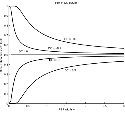
It can be inferred from Equation 2.9 that there are multiple values ofwandθ that will
result in the same value of DC and, therefore, produce the same distortion on an isolated
edge [11]. Figure 2.3 shows an multiple DC isocline plots for different DC values. The
−3 −2 −1 0 1 2 3 4 0
0.2 0.4 0.6 0.8 1
ESF(x/w1)
ESF(x/w2)
DC
θ1
θ2
the plot of the isocline DC lines that the DC lines extend over the entire range ofwandθ
values.
0 0.5 1 1.5 2 2.5 3
0 0.1 0.2 0.3 0.4 0.5 0.6 0.7 0.8 0.9 1
PSF width w
Binarization threshold theta
Plot of DC curves
DC = −0.5
DC = −0.1 DC = 0
DC = 0.1
DC = 0.5
Figure 2.3: Edge spread degradation parameter DC isocline lines for DC values -0.1, -0.5, 0, 0.1 and 0.5.
2.1.3 Stroke Spread, Modified Delta C (MDC)
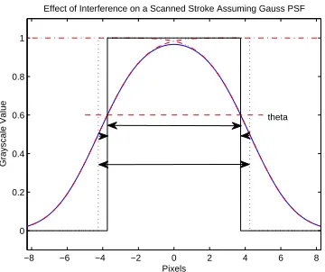
In the previous subsection, we discussed the effect of scanning on isolated edges. In this
section, we will discuss the effect of scanning on pairs of adjacent edges, also knows as
strokes. Character images contain many edges like this. Scanning changes the thickness of
these strokes. This change in thickness is not the same as the shift predicted for isolated
edges because the opposite edges in the stroke interfere with one another. This effect was
analyzed and formulated mathematically by McGillivary in his thesis [9]. If the edges are
parallel, the one dimensional cross section of a scanned stroke is a square pulse with a
widthτ. Let us assume that the square pulse is centered at the origin. In this case, the value
s(x) =s(−x) =ESF
τ−2x
2w
−ESF
−τ−2x
2w
. (2.10)
Similar to the scanned edges, the new edge locations occur wheres(x)is equal toθ. Let
us denote the thickness of the stroke after thresholding byτscanned, and if it is found to be
greater than zero, then the threshold is given by
θ =ESF
τ−τScanned
2w
−ESF
−
τ−τScanned
2w
. (2.11)
The change in stroke thickness MDC can be defined as
τscanned=τ+MDC, (2.12)
which leads to
θ =ESF
− MDC 2w −ESF −2
τ−MDC
2w
. (2.13)
As the τ value gets bigger, Equation 2.13 becomes
θ =ESF
−
MDC
2w
. (2.14)
When τ is large enough to make the edges independent, the change in stroke thickness
becomes twice the DC.
In addition to the occurrence of change in stroke thickness, there is also a chance that
a stroke will disappear altogether. This will occur at instances when the threshold exceeds
the maximum value ofs(x). The value of threshold selected affects the image in the sense
that a higher threshold value ensures fewer black pixels in the resulting image and vice
−8 −6 −4 −2 0 2 4 6 8 0 0.2 0.4 0.6 0.8 1
Effect of Interference on a Scanned Stroke Assuming Gauss PSF
Pixels
Grayscale Value
theta
Figure 2.4: When a stroke characterized by two parallel edges is scanned, the resulting stroke thickness changes. Interference between the parallel edges causes the grayscale value of pixels to be less than that predicted by the ESF. As a result, the stroke thickness will be less than that predicted by DC.
θmax=ESF
τ 2w −ESF − τ 2w
=1−2·ESF
− τ
2w
. (2.15)
First it must be verified if θ is greater than θmax by using Equation 2.15. If it is, the
stroke vanishes. Once this is verified, the upper and lower bounds on values of MDCare
set. These bounds are
MDC>−τ, (2.16)
and
MDC≤2·DC. (2.17)
Thus, we can state that at largerτ values
DC= MDC
2 . (2.18)
The lower bound limits on the value of MDC comes from the fact thatτScanned cannot
ESF is always positive. For a given set of values forτ,w, andθ, it is possible to determine
the value of MDC. The maximum and minimum bounds on the value of MDC value are
calculated, and interpolation is done between the maximum and minimum values of MDC,
indicated by Equations 2.16 and 2.17, respectively, to estimate the MDC value.
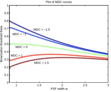
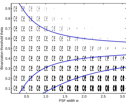
Similar to Figure 2.3, which depicts an isocline plot of many DC values plotted on
the same graph, Figure 2.5 shows multiple MDC isoclines drawn simultaneously. The
important aspect that is visible instantly is that the plots of DC and MDC lines do not
match. The MDC curves slope down as PSF width increases in comparison to DC lines.
PSF width w
Binarization threshold theta
Plot of MDC curves
1 1.5 2 2.5 3
0 0.1 0.2 0.3 0.4 0.5 0.6 0.7 0.8 0.9 1
MDC = −1.5 MDC = −1
MDC = 0
MDC = 1
MDC = 1.5
Figure 2.5: Edge spread degradation parameter MDC Isocline lines for MDC values -1.5, -1, 0, 1, and 1.5.
2.2
Clustering
Clustering is a method of classification that groups data with similar features. In pattern
recognition, we try to find elements sharing a region in the feature space, because elements
of a particular class will generally lie closer to each other. Since labeling each feature
without the knowledge of their class. Once such clusters have been formed, it is easier to
label the clusters and perform any error analysis. There are many clustering algorithms
used in pattern classification. The following subsections talk about the Isodata or C-means
clustering and Fuzzy C-means clustering algorithms used in this thesis.
2.2.1 Isodata Clustering
Isodata stands for Iterative self-organizing data analysis technique. This is also sometimes
called C-Means. Isodata is the algorithm used to cluster the characters in this thesis. The
first step is to decide into how many clusters, C, the data needs to be divided. This algorithm
works by first randomly selecting C points from the dataset, depending on the desired
number of clusters, as means. These will be the means used to group the data. After the
mean values have been selected, data is grouped into clusters. To cluster the data, a 1
nearest neighbor method was used. Distances are compared from the C randomly selected
means to find the points in the dataset closest to these point means in consideration and
adding the closest points to the respective cluster to which these mean points belong. After
every iteration, the cluster means are updated based on points associated with the means
in the previous iteration. Then, all the points are again associated with the new means
and this iterative approach continues until none of the cluster means change. The point at
which none of the means change tells us that the datapoints have been grouped as close to
the cluster center as possible.
2.2.2 Fuzzy C-Means Clustering
Fuzzy C-means (FCM) is a data clustering technique in which a dataset is grouped into C
clusters with every datapoint in the dataset having membership in every cluster partition
its values measure degrees to which objects satisfy imprecisely defined properties, which
in our case is the cluster assignment of a point. The membership of a point in a particular
cluster partition is inversely proportional to the distance from the cluster partition. Consider
the two examples that follow to understand this concept of membership. First consider a
certain datapoint that lies close to the center of a cluster partition, it will have a higher
degree of belonging or membership to that cluster partition than in other cluster partitions.
Next consider another datapoint that lies far away from the center of a cluster partition;
it will have a low degree of belonging or membership to that cluster partition and greater
membership to a neighboring cluster partition it lies closer to.
The logic of this algorithm starts with first deciding on the final number of clusters, C,
followed by an initial guess for the cluster partition centers, which are intended to mark
the mean location of each resultant cluster partition. The initial guess for these cluster
partition centers is most likely incorrect. The next step in the algorithm is to assign every
datapoint a membership grade for each cluster partition randomly between 0 and 1, then
compute the centroid for each cluster partition followed by computing the membership
function for each point of being in the cluster partitions. The calculation of centroid
and membership function is repeated until the algorithm has converged (i.e., the change
in coefficients between successive iterations is not more than a small value referred to
as the sensitivity threshold). By iteratively updating the cluster partition centers and the
membership grades for each datapoint, this fuzzy C-means algorithm iteratively moves the
cluster partition centers to the right location within a dataset. This iteration is based on
minimizing an objective function that represents the distance from any given datapoint to a
cluster partition center weighted by that datapoint’s membership value [14, 15, 16].
The mathematical description of the algorithm is described in the following discussion.
of all points in that cluster partition and weighted by the membership value of the points,
is given by
centerk= ∑xmk(x)
fx
∑xµk(x)f
. (2.19)
The degree of class memberships is calculated as
µci(x) =
k
∑
j=1
µci(x)·
1
km−mjk
2
(f−1)
1
km−mjk
2
(f−1)
, (2.20)
where m1, m2,...., mk denotes the k nearest neighbors of x, and f is referred to as the
fuzziness parameter. The value of f determines how heavily the distance is weighted
when calculating the class membership. Looking at the equation, we can conclude that
as the value of f increases, all the neighbors are weighted more evenly and when the
value off decreases, the closer neighbors are weighted far more heavily than those farther
away. Consider a test point xdivided into 2 partitions C1 andC2 using FCM, which has
membershipsµ1andµ2for the 2 clusters. The sum of the membership function values for
a point in all clusters always adds up to 1: i.e.,
µ1x+µ2x=1. (2.21)
2.3
Classifiers
After the dataset is divided into homogeneous partitions, the next step involves the design
of a classifier to evaluate if the division of the dataset had any effect on the classification
vital points that have to be evaluated before the selection of a classifier is made are the
ease of implementation, training time, and performance. A few classifiers that are widely
used are Neural Networks, KNN, and others. The Bayesian classifier was used to evaluate
the classification accuracy of the methods explored in this thesis. The Bayesian classifier
was mainly used due to its statistical accuracy and ease of implementation. Section 2.3.1
explains in detail the concept on which a Bayesian classifier classifies test points.
Bayesian classifiers belong to the class of crisp classifiers as the output results receive
a single class label. The Bayesian implementation can be manipulated to include a fuzzy
method in order to give some flexibility in classification of a test point. In this thesis,
different combinations of training and testing approaches have been implemented to design
the classifier to divide and classify the dataset. The dataset is still being divided by the DC
and MDC degradation parameter values, and in addition they have different combinations
of fuzzy and crisp training and testing methods. The various combinations that have been
implemented are crisp training of the dataset divided by DC and MDC followed by crisp
testing, crisp training divided by DC and MDC followed by fuzzy testing, fuzzy training
divided by DC and MDC followed by crisp testing, and fuzzy training divided by DC and
MDC followed by fuzzy testing. Sections 2.3.2 through 2.3.5 will discuss, in detail the
approaches and implementation of the four approaches mentioned above.
For sake of simplicity of understanding and implementation, the division of data by a
single DC and MDC value into two partition is being considered for experimentation and
computing results. The same explanation and reasoning can be extended to the case for
2.3.1 Bayesian Classifier
The Bayesian classifier has its roots in statistical pattern recognition. It is a simple
prob-abilistic classifier based on applying Bayes theorem, which is based on independence
assumptions. In simple terms, a naive Bayesian classifier assumes that the presence (or
absence) of a particular feature of a class is unrelated to the presence (or absence) of
any other feature. “For example, a fruit may be considered to be an apple if it is red,
round, and about 4diameter. Even though these features depend on the existence of the
other features, a naive Bayes classifier considers all of these properties to independently
contribute to the probability that this fruit is an apple” [12]. In spite of their naive design
and apparently over-simplified assumptions, naive Bayes classifiers have worked quite well
in many complex real-world situations. Depending on the precise nature of the probability
model, the naive Bayes classifiers can be trained very efficiently in a supervised learning
setting. An advantage of the naive Bayes classifier is that it requires a small amount of
training data to estimate the parameters (means and variances of the variables) necessary
for classification.
The Bayesian classifier assumes that the prediction of a character class can be modeled
using any of the known distributions like Gaussian, Cauchy, etc. It must be noted that with
the choice of different distributions, the discriminant function form will change based on
the selected distribution. In this thesis, the Gaussian distribution was selected and it uses
the center and spread of the feature vectors of the character class. The decision criteria
can be influenced by the relative frequency of a particular class. The Bayesian classifier
uses a discriminant as the metric to determine to which class a test character belongs.
The following discussion will give details about the discriminant function and probability
discriminant for each character class,i, is given by [13]
gi(x) = −1
2 (x−mi)
T
Σ−i 1(x−mi)−
d
2ln(2π)−
1
2ln|Σi|+ln(P(wi)), (2.22)
wheremi,d, andΣiare, respectively, the means of the character class under consideration,
the number of features, which is considered a constant and covariance values for the
character classes in the training dataset. The class,i with the greatest discriminant value,
gi(x), for test point, x, is chosen.At everytest point, the mean and covariance values of
each character class in the training dataset are used to evaluategi(x), and the test point is
assigned to the character class that yields the maximum value for this parameter.
In our case, all the class probabilities,P(wi), are equally likely because all classes have
an equal number of characters in the test set. If the dataset is generated synthetically in
such a way that the probability of selecting either character class in a data set is equal, this
probabilityP(wi)can be ignored because it doesn’t affect the relative values of Equation
2.22 for different i. The 2π term can be ignored because it is a constant value and will
remain the same in the calculation of discriminant values of either class and thus can be
neglected. Thus, Equation 2.22 can be simplified to
gi(x) = −1
2 (x−mi)
T
Σ−i 1(x−mi)− 1
2ln|Σi|. (2.23)
Equation 2.23 gives the hypothesis of aposterior probability of the test point belonging
to a certain class. The Bayesian Classifier assigns the unclassified character to the character
class that has a higher value from the application of Equation 2.23. This is what was used
2.3.2 Crisp Training
Crisp training refers to the training approach in which the training parameters for each
character class are calculated for a rigid case where the point belongs to a definite cluster
partition group. For ease of understanding the implementation approach, the case when
a dataset is divided into two partitions has been elaborated. In this classifier training
implementation, the training dataset is divided into 2 partition datasets by using DC and
MDC degradation parameter values, respectively. Points will belong to one partition or the
other, but not both. The training dataset points from the first partition are used to calculate
the covariance matrices,Σi,and means, mi,and then we proceed to calculate these values
for the second partition. Calculating these parameters comprises the crisp training process.
These parameters will then be used to calculate the discriminant function values when a
test point is classified using Equation 2.23.
2.3.3 Fuzzy Training
Fuzzy training refers to the training approach in which the training parameters for each
character class are calculated for a non-rigid case where the point may belong partially to
multiple cluster partition groups. Every datapoint has a membership value in each of the
resultant partitions whose value is determined by the probability of the point belonging to
that partition. The total of memberships for a point in all partitions always adds up to 1. The
membership function values are obtained from the fuzzy C-means clustering algorithm. In
this implementation, the training proceeds similar to the method described in Section 2.3.2.
The only change that we see in the training is that the features of the training dataset in each
partition when divided by DC and MDC values are scaled with the membership values in
moment feature of a datapoint with the membership values. This is done for every point of
the training dataset. These scaled training dataset points from the first partition are used to
calculate the covariance matrices,Σi,and means,mi,and then we proceed to calculate these
values for the scaled training points in the second partition. Calculating these parameters
comprises the fuzzy training process. These parameters will then be used to calculate the
discriminant function values when a test point is classified using Equation 2.23.
2.3.4 Crisp Testing
Crisp testing refers to the testing approach in which the unclassified test point is estimated
based on determining the discriminant function value while rigidly belonging to a particular
cluster partition or group. The test datasets are divided into two partitions based on a
DC or MDC value. For testing individual test points in either partition, the discriminant
value is calculated with Equation 2.23 using the training parameters from the corresponding
partition in the training set. The discriminant values are calculated for the test point being a
‘c’ or an ‘e’. The test point is assigned to the character class that has the larger discriminant
value of the two values.
2.3.5 Fuzzy Testing
Fuzzy testing refers to the testing approach in which for every unclassified test point, all the
determinant function values are calculated for all possible partitions and this is scaled with
the appropriate membership function and a decision is made. Consider the case in which
the training dataset is divided into two partitions C1 and C2. In this approach of testing, we
do not divide the test datapoints into partitions using crisp degradation parameter values and
subsequently use the corresponding training parameter values to calculate the discriminant
for each test point using training parameter values from both the partitions. The test patterns
belong to either of the character classes ‘c’ or ‘e’ represented byi=1 for the test point of ‘c’
andi=2 for an ‘e’. A dataset that comprises of ‘c’ and ‘e’ and divided into 2 partitions C1
and C2 has 4 possible discriminant values for a test point. These 4 discriminant values are
the test point belonging to partition 1 (C1) and being a ‘c’ i.e. i=1, test point belonging to
partition 1 and being an ‘e’ i.e. i=2, test point belonging to partition 2 (C2) and being a ‘c’
i.e.i=1, and test point belonging to partition 2 and being an ‘e’ i.e. i=2. For calculating the
four partition specific probabilities, the training parameters from the respective partitions
of the training set are used. These discriminant values are scaled with the respective
membership values of the test point in each of the two partitions. A modified discriminant
value
gi−f uzzy(x) =giC1(x)·µ1+giC2(x)·µ2 (2.24)
is calculated twice for each test point. In the equation,gi−f uzzy(x)is the total discriminant
function value for the character point summed across both the partitions, and µ1 and
µ2 are the membership values for the test point character in C1 and C2, respectively.
Initially, the discriminant function of the test point of belonging to character class ‘c’ and
partition 1, i.e. giC1(x),followed by being a ‘c’ and belonging to partition 2, i.e. giC2(x),is
evaluated. These values are scaled with the membership function valuesµ1and µ2 in the
respective partitions. This equation value is similarly evaluated for the test point belonging
to character class ‘e’. The resultant scaled discriminant function values of characters ‘c’
and ‘e’ in C1 and C2 are added to get the resultant discriminant values of the test point
being a ‘c’ and an ‘e’ in both partitions.
Equation 2.24 is a slight variation of Equation 2.23 used for evaluation in crisp testing.
In the crisp classification case, a point belonging to partition 1 will have membership of 1
in C1 and 0 in C2 unlike a fuzzy case in which test points have partial memberships where
membership function µ has values between 0 and 1 but never 0 or 1. Thus, in the fuzzy
case, the probability calculation before a test point is assigned does not just limit itself to
one partition that is determined crisply but values are calculated by considering the test
CHAPTER 3
EXPERIMENTS
The tests that were implemented in this thesis were motivated by the goal to explore and
answer the following six questions. These questions are:
1. Did the division of the dataset improve the accuracy of classifying the dataset?
2. Is MDC a better parameter to partition the dataset than DC?
3. If the dataset was divided by the incorrect DC and MDC values, how does it affect
the performance?
4. What is the reasonable number of partitions into which a dataset should be divided?
5. What is the error associated with estimating the wrong DC and MDC parameter for
a character?
6. Does the use of a fuzzy approach of classification offer any improvement in
perfor-mance over the crisp approach?
Before these questions can be explored, the first step was generating synthetic data similar
to degraded scanned characters. The data used to explore this is described in Section
3.1. Some of the characters produced will vanish, and some will be excessively degraded.
The degraded synthetic dataset generated has to be visually inspected to decide what is
based on visual appearance of the degraded character. In Section 3.2, the preprocessing of
the data, which includes filtering for removing isolated salt and pepper noise and limiting
exploration to characters with a minimum number of pixels, will be explained.
After the dataset was generated, the datapoints that varied in character stroke thickness
were grouped into similar featured classes using the Isodata clustering algorithm. This
clustered data was then partitioned into smaller homogeneous datasets using the edge
spread degradation parameters DC and MDC as the division parameters. This was done
in order to facilitate the generation of smaller training datasets with similar degradations.
Finally, this divided data was used to train and classify datasets to verify if the partitioning
made any change to the classification accuracy compared to an undivided dataset.
Subsec-tions 3.3.1 through 3.3.3 discuss the Isodata clustering, boundary fitting, and division and
classification tests. With all the requirements fulfilled to analyze the tests for this thesis,
the following briefly discusses the implementation details.
To answer the first two questions, tests were done on the unpartitioned dataset as well as
the dataset divided by an exhaustive set of DC and MDC values, each with the subsequent
classification details of which are given in Section 3.3. Question 3 analyzes what happens
if we use an incorrect value to divide the dataset after we do the clustering or we just
make an educated guess on the parameter to partition the division value. Section 3.5
discusses the implementation of accuracy analysis done for the different values of edge
spread degradation parameters and how that affects the accuracy as we move across the
clusters.
Question 4 explores whether there is an upper limit on the final number of partitions.
Division of the dataset into more partitions to improve the classification may not always
hold true and there might exist a limitation on this approach. Section 3.4 discusses how the
Questions 1 through 4 analyzed classifier performance based on the assumption that
the points were assigned to the correct partitions. The training datapoints are divided
into groups based on the DC and MDC values calculated from the degradation parameter
estimated from the character. Questions 5 and 6 analyze what happens when the
degra-dation parameters estimated for a character are incorrect. The effects as well as possible
implementations of solutions to overcome this problem are discussed in Section 3.6.
3.1
Dataset
The scanner model was used to synthetically generate datasets comprised of characters
‘c’ and ‘e’ with varying PSF widths w and binarization threshold θ. In this case, only
the characters ‘c’ and ‘e’ were chosen in the experiments because they look very similar
and hence statistically have similar properties.Thus, differentiating between them poses the
greatest challenge to modern OCR engines. Once the idea and method suggested in this
thesis yield good classification accuracy for ‘c’ and ‘e’, the same concept can be extended
to datasets ‘a’ through ‘z’ in different fonts and font sizes.
The dataset used in the experiments in this thesis contains a total of 100,000 characters.
The characters that are used in the experiments have been generated by using the
degra-dation model [11] with random Gaussian noise included in the data generation to account
for the noise that a character is degraded by in real-text scanning. The characters that
are generated are 12 point, 300 dpi, sans serif font, lowercase characters ‘c’ and ‘e’. The
PSF width used for blurring ranges within the limits 0.2 to 3. Scanning introduces noise
in the resultant transcript of scanned characters in digitized form. This noise has to be
accommodated or simulated while the classifier is trained to get better classification. It can
scanned character and almost zero or no noise pixels around the character that is scanned.
While generating the character dataset, Gaussian noise with standard deviation up to 0.15
was added in the generation. The blurred characters with noise included that have been
generated have to be thresholded to get the final character image. The threshold is also
chosen randomly between the limits 0.05 and 0.95. Any character pixel value below this
threshold value is considered to be white or background.
After thresholding, the character is passed through a filter that removes all the salt and
pepper noise that is not directly associated with the character and is present in the image
background. This pre-processing is done because the moment features are to be calculated
on the character and not separate disjoint noise. The filter to remove salt and pepper noise
looks for standalone single pixels that are present with a gap of 1 pixel around them and
removes them. At times, the noise pixel is attached to the character pixel and hence cannot
be filtered by this approach. This noise is referred to as edge noise and is not removed in
this thesis. Looking at Figure 3.1(a), which has noise, it can easily be concluded that the
character generated is noisy with uncorrelated noise. Filtering has been done to ensure that
we are only considering the noise that exists at the character corners or along the boundary
of the character stroke so that they visually resemble the noise introduced in a character by
an actual scanning process. Figure 3.1(b) shows the character ‘c’ without salt and pepper
noise. There is no skew added to these generated characters as the only degradations that
are being considering in this thesis are edge spread degradation parameters DC and MDC
introduced due to scanning operation. Features can be calculated that are skew independent.
The synthetic data images with the majority of salt and pepper noise removed are
then used to extract the features used for classification. The features chosen are moment
features. The moments can be defined as features of an object that allow a geometrical
(a) (b)
Figure 3.1: (a) Character ‘c’ with noise, (b) filtered image with most of the noise around the image removed
features for a gray value functionf(x,y)of an object are given by
mp,q=
Z Z
xp·yq·f(x,y)dxdy, (3.1)
and
µp,q=
Z Z
(x−x¯)p·(y−y¯)q·f(x,y)dxdy. (3.2)
where ¯xand ¯yare the moment featuresm0,1andm1,0. This integration is calculated over the
area of the object. If we use binary images, the gray value functionf(x,y)becomes
f(x,y) =b(x,y). (3.3)
Moments are generally classified by the order of the moments. The order of a moment
depends on the indices pand qof the moment mp,q. The sump +q of the indices is the
order of the momentmp,q.Thus, the zero order moment, i.e. (p,q)= (0, 0), is given by
m0,0=
Z Z
b(x,y)dxdy. (3.4)
the number of pixels in the image. The first order moments, i.e. (p,q) = (1,0) or (0,1), are
given by
m1,0= Z Z
x·b(x,y)dxdy, (3.5)
and
m0,1=
Z Z
y·b(x,y)dxdy. (3.6)
The first order moments contain information about the center of gravity of the image.
In this thesis, the moment features that are extracted arem0,0,µ0,2,µ1,1,µ0,3,µ2,0,µ3,0,
µ2,1, and µ1,2. These 8 moments will be the features used to train and test the classifier.
These 8 moment features are calculated for each of the characters in the dataset.
3.2
Analysis of Cutoff Selection for the Number of Pixels in Generated
Characters
With the degradation being simulated, character strokes can get very thin and sometime
characters can vanish all together. Equation 2.15 explains mathematically the condition
under which a scanned stroke may completely disappear. Thus, it becomes necessary to
decide what is a permissible degradation for a character in the dataset so that it still has
significant analysis capability. This is done by deciding how many pixels the generated
synthetic degraded character must have relative to the ideal character. This is a vital
decision that sets the limits on the level of degradations that are used in training the
classifier. Degraded characters with negative DC or MDC values can thin strokes to just
stroke widths can be seen in Figure 3.2. In case there are only a very few pixels, it is
insufficient or impossible to conclude even visually if it is a ‘c’ or ‘e’, which makes it
difficult if not impossible to recognize using recognition algorithms. We need to select a
value for the minimum number of points a character must maintain. This decision was
made after visually inspecting an ideal character and different variations of it with varying
numbers of black pixel counts.
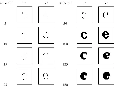
In order to do this analysis, an ideal character using a PSF width of 1 and thresholded
at 0.5 was generated. The number of black pixels in this ideal character was calculated.
Synthetic characters that have the total number of pixels varying between 5% and 150% of
the ideal character pixel count were generated. These generated characters were visually
inspected to decide which of these characters are visually identifiable and hence can be
considered part of the dataset.
In earlier work [8], characters with as few as one black pixel were included in the
dataset. The intuitive feeling before we start off with analyzing the cutoff value selection
is that the more pixels we have, the better we can conclude visually what character we are
seeing. This in turn leads to more comprehensive features being fed to the classifier. This
ensures minimal misclassification. However, since the effect of degradation on recognition
is being evaluated, characters that are largly eroded are also of interest. In most cases, it can
be noticed that there are always partial characters but never just a single dot, few dots or
clusters of very few pixels. The worst case that we encounter is probably a partially eroded
printed character that leads to a partial scanned character. Figure 3.2 shows characters
‘c’ and ‘e’ with cutoff values between 5-150% on number of pixels relative to an ideal
character.
As we successively lower the pixel cutoff as we go from 100% down to 5%, we can see
up just as a few dots without any definite shape and hence we cannot visually conclude
what character it is. In case we extract the moment features from such characters and used
them to train and classify, we will not be able to get very good classification due to lacking
data sufficiency. Hence, we need to increase the cutoff selection to get visually classifiable
characters. The selection of cutoff is totally a visual choice. The data is generated for a
particular cutoff value, data is visually inspected for data sufficiency and then a value is
selected. After looking at Figure 3.2, we concluded that selecting 10% cutoff will produce
a good dataset with manageable degradations.
% Cutoff ‘c’ ‘e’ % Cutoff ‘c’ ‘e’
5 50
10 100
15 125
25 150
3.3
Implementation Details to Validate the Tests
The same data are used for all experiments. Three parameters that are calculated from
the training file and used to classify the test points are the class conditional means and
covariances and the root mean square (RMS) values for each feature. The mean and
covariance values were used to calculate the probability value of each test point being any
of the character classes to classify them. The RMS value is defined as a statistical measure
of the magnitude of a varying quantity. The moment features calculated for the character
points are not in the same range (i.e., a few features are very small while others features are
large). In order to calculate the 1 nearest neighbor from the mean, equal importance has to
be given to each feature of the 8 to estimate the nearest neighbor. This is possible only if
the value of all the features are comparable which is achieved by getting them in the same
relative scale. RMS values are needed so that the test points can be normalized based on
the training set values. The Bayesian classifier is used to classify the datapoints in all the
experiments.
The 10 fold cross validation approach is used for all experiments. After testing all the
test points, error values of the classification results were used to calculate the weighted
percentage classification error. In this calculation, the errors in each partition are scaled
with the weight of that partition (i.e., the total datapoints).
The ultimate goal in using an OCR engine is to get minimum error in the final digitized
transcript. This can only be achieved if the training is done in such a way that most of
the test patterns to which the OCR engine will be exposed are used in the training phase.
The idea of dividing the non-homogeneous dataset into smaller homogeneous sets based on
division by the DC and MDC degradation parameters is a very effective method to train the
![Figure 2.1: This scanner model is used to determine the value of the pixel f[i,j] centered oneach sensor element[10].](https://thumb-us.123doks.com/thumbv2/123dok_us/8925513.1845321/23.612.129.524.495.619/figure-scanner-model-determine-centered-oneach-sensor-element.webp)