CRL 91 2 pdf

1"1', r": r, J:J2:

p

VOl - A Visual Debugging Interface

for Image Interpretation

and Other Applications

Gudrun Klinker

Digital Equipment Corporation Cambridge Research Lab

CRL91/2

Abstract

March 7, 1991

HPL/RE.SEAHCH L1BRARV

BUILDING #2L

P 0 80X1O~90

PALO ALiO. CA 94303-09'11

Higher-level image interpretation systems typically consist of many tightly-coupled modules, each related to a particular aspect of the interpretation task. When such a system produces wrong results, programmers generally spend a lot of time writing special-purpose display rou-tines to facilitate investigating the problem. This paper presents an attempt at unifying such ef-forts by merging graphics programming with debugging technology. Several generalizations are necessary to provide useful general-purpose display mechanisms: 1) The mechanisms need to be highly interactive such that programmers can select and change display preferences at de-bugging time. 2) The display routines should not be restricted to traditional, two-dimensional images. 3) The programmer must be able to visualize the data-dependent relationships between modules. VDI is a general-purpose Visual Debugging Interface designed to provide these gen-eralizations. It is highly interactive, operates on arrays of arbitrary dimensionality, and provides mechanisms to describe dependencies between the results generated by various interdependent modules.

Keywords: interactive array visualization, scientific visualization, computer graphics, computer vision, debugging aids.

Contents

1 Introduction 1

2 The Interactive Interface 3

2.1 Data Selection 3

2.1.1 Data Slicing, Cropping, Subsampling and Thresholding 4

2.1.2 Links between Several Arrays 5

2.1.2.1 Direct Restrictions 6

2.1.2.2 Indirect Restrictions 8

2.1.2.3 Displaying several linked arrays together 12

2.2 Data Display 12

2.2.1 Arrangement of Information in a VOl-Window 12

2.2.2 Interpretations of Mouse Buttons 13

2.2.3 Graphical Representations of Arrays 14

2.2.3.1 Intensity-based displays 14

2.2.3.2 Graphs (terrain maps) 15

2.2.3.3 Printed numbers 18

2.2.3.4 Combinations of several graphical representations 22

2.2.4 Overlays of symbolic data 23

2.2.5 Display Styles 24

2.3 Data Manipulation 26

3 The Program Interface 28

4 Other Applications for VOl 30

5 Summary 32

Acknowledgments 33

References 34

Figures

Figure 2-1 A time sequence of color images 3

Figure 2-2 A subsampled color image 4

Figure 2-3 VOl's menu for linking arrays 5

Figure 2-4 Direct restrictions on an array 7

Figure 2-9 An x-y-based layout of printed numbers from a color image 19

Figure 2-10 A y-based layout of printed numbers from a color image 20

Figure 2-11 A null-based layout of printed numbers from a color image 21

Figure 2-12 Printed numbers for an inter-reflection area in the color image 22

Figure 2-13 Graphical overlay of symbolic data on an array 23

Figure 2-14 VOl's menu for selecting display styles 24

Figure 2-15 Graphical interface to change color maps 25

Figure 2-16 VOl's menu of data manipulation operations 27

Figure 3-1 Example: Program to invert a two-dimensional image 29

Figure 4-1 VOl as a tool for visualizing constraints between parallel processes on a

1 Introduction

For many years, it has been common practice for computer vision labs to develop their own graphics libraries - tailored to their specific hardware environment. With the advent of window system languages and graphics packages [Scheifler and Gettys 86, Gettys et al 90, GKS-3D 87, PHIGS 87], several general-purpose toolkits for viewing images and volumetric data have emerged from computer graphics research [XVision 3.0 89, VoxelView 89, Upson et al. 89]. Some of such visualization systems provide the basic mechanisms for displaying and slicing two- and three-dimensional data blocks and for rendering geometric data. Augmented with a (user-extensible) library of image processing routines and with an interactive visual program-ming mechanism, they are powerful toolkits for perforprogram-ming a sequence of image processing steps on images. They are designed to be used by (non-programming) scientists who use the toolkit as an aid for enhancing/visualizing images such that they (the humans) can interpret them more easily.

But such toolkits seem to be of limited usefulness to computer vision researchers who are trying to write automatic image interpretation programs. The basic (visual programming) assumption of the toolkits is that image processing operations can be packaged into independent "black-box" modules with easily specifiable input/output behavior and that the image data flows through a network of such modules. This is often the case in low-level image processing tasks. But in image understanding systems, the modules generally don't operate that independently of one another [Hanson and Riseman 78, Klinker et a1. 90]. Consider the example of an object rec-ognition algorithm that needs to detect the boundaries of an object in an image. The object may be as complex as a house, consisting of several walls, windows, doors, a roof etc., and it could be viewed from any angle, even be partially hidden behind trees, cars or other houses. Object recognition has to account for such possibilities and exploit partially gathered evidence to build up a consistent interpretation of the entire scene. Such evidence is stored partially in arrays ac-companying the original image (such as a segmentation image) and partially symbolically (for example as a region list describing the shape and other properties of the currently segmented regions). Progress in some modules (e.g., for detecting windows) may be tightly coupled with progress in other modules (e.g., for detecting walls). Accordingly, image understanding mod-ules can depend in very complex and global ways on the overall state of the interpretation. Blackboard systems have been suggested as one useful communication scheme between mod-ules [Hanson and Riseman 78, Draper et a1. 89, Goto and Stentz 871. The current visual pro-gramming paradigm does not support such tight coupling between modules. It would be ineffi-cient to pass the contents of the entire blackboard between modules. Furthermore, the blackboard paradigm assumes that the various vision modules operate in parallel: every module is an independent agent that sits and waits until some information on the blackboard triggers its interest. This scheme of a static and global arrangement of agents and data stands in contrast to the dynamic data flow concept adopted in visual programming.

individ-mers could interrupt the program execution at arbitrary places and visualize the current state of the image interpretation process.

This paper presents an attempt at merging graphics programming with debugging technology. To provide general-purpose interactive graphical display routines for arrays, some common dis-play practices haveto be extended. This paper discusses such generalizations. It is essential that the interactive mechanisms match the necessities of the underlying program modules to access many images that depend on each other. That means that if the window detection module de-pends on (partial) results produced by the wall detection module, then the visual debugging in-terface must provide mechanisms for viewing the data under such constraints. For this purpose we provide mechanisms to formulate relationships between pixels in different images. The pro-grammer can, for example, request to view all those pixels of the original image which the wall detection module has already labeled as being potential wall candidates.

A vision research workbench, "KBVision", with similar goals appeared several years ago [Stephenson 90]. However, this system was only designed to address the needs of visualizing two-dimensional images. We extend the display capabilities from the traditional two- or three-dimensional image domain to arrays of much higher three-dimensionality because programming lan-guages provide arrays of higher dimensionality and debuggers should reflect that concept. With this extension, not only the traditional image-oriented applications can benefit from the debug-ger's display capabilities but any program that operates on arrays. Most current work in com-puter vision uses two-dimensional images or sets of two-dimensional images. So far, it is most common to display the data as two-dimensional (x,y)frames, while providing specialized exten-sions for representing a third dimension (pseudo-coloring, stereo glasses, movie-loops). But we expect that the displaying needs will change in the future: Some applications exist already now where researchers prefer to view the data along other dimensions, e.g., to display (x,time) slices of an image sequence [Bolles and Baker 85, Adelson and Bergen 86]. Other applications need to visualize three-dimensional data volumes [Carlbom et al 91, Klinker et al. 90, Szeliski 90, Szeliski 91]. Furthermore, we expect that research in different fields of computer vision will become more integrated in the future and that image data will then comprise more than three dimensions. Image data could, for example, be a (five-dimensional) time sequence of stereo color images, with different image understanding modules operating on different slices (color, stereo or time) through the data volume. At that point, it will be most useful to think of image data as a high-dimensional array with no preferred axes and let the programmer select viewing and accessing preferences interactively.

2 The Interactive Interface

We have divided interactive input into three classes of commands: commands for 1) specifying data selection criteria, 2) defining data manipulation techniques, and 3) defining the display style. Each of these sets will now be described in detail.

2.1 Data Selection

VDI operates on multi-dimensional arrays for which each dimension is described by a feature

axis. Figure 2-1 shows an example of a four-dimensional array: a (time) sequence of color

im-ages with

x,

y, the color vector,

c,

and the time vector,

t,

defining the feature axes.

High-dimensional arrays generally cannot be displayed in their full dimensionality. VDI pro-vides an interactive interface through which the programmer can slice the data along arbitrary dimensions. The interface also possesses basic cropping and thresholding capabilities, such that the programmer can restrict data access to a subarea and a subrange of values. Finally, the inter-face provides mechanisms for relating data selection from one array to the values of data ele-ments in other arrays. Such mechanisms allow the programmer to issue a command like "select all pixels from image i which belong to region r (i.e., whose region label in the related segmen-tation imagej isr)".

(

I

I

I

I

I

Y

I

<,

--~

I I

-+.::.,

I

I _I

I _I

--~

I _I

I _{I I}

t»;

I I I

-~---I _{I Iy}

I _{I I}

I contained feature

t=3

<,

I_I II II values (r,c) at framing

I I I

position [x.,y ]

t=2

<,

I_I I_I 1 J

I I

t=1

<,

I_I

I ~

2.1.1 Data Slicing, Cropping, Subsampling and Thresholding

VDI's data slicing mechanism distinguishes between two kinds of features: framing features

and contained features. The framing features are those by which the programmer defines a

frame for a slice through the data. The contained features are the remaining (i.e., non-framing) features. Figure 2-1 shows a typical arrangement for viewing a time sequence of color images as a sequence of two-dimensional image frames:

x

and y are the framing features, with each (x,y)-position containing the various pixel values along the color and time dimensions. Any par-ticular image frame represents a slice through the 4D data block, with fixed values for t and c and varying values for x andy.

x

=

256

y

=

256

(115, 30, 18)

47~

[image:8.612.36.566.205.519.2]

Done [0 ..479] ...

::1:II~1r~dW.f~1U:::g~~HU~::::ij:~:::':.~n9~(:

6!l6il

StartVal [0.. 478]

q

Data Selection Parameters:

Select

*

All vectors

!II

color: [0,2] ++1 of "cimg" in frame

o

y : [0,478] ++2

Ox:

[0,510] ++2

with values [0 255]

Figure 2-2 A subsampled color Image

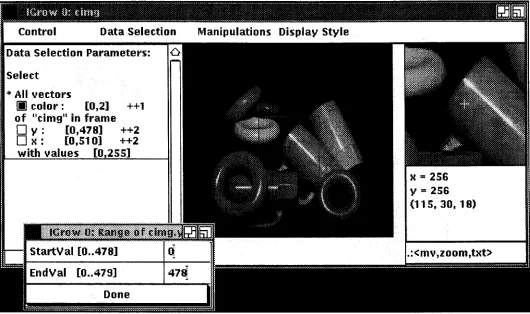
Figure 2-2 shows a sample interaction with VDI1. The center area displays a subsampled color

image of a scene of plastic cups and donuts? The area to the left presents the current values of the data selection parameters. Each feature axis is listed with its currently selected range of val-ues (in square brackets) and its subsampling increment (here: ++1 or ++2). VDr provides the interactive tools for slicing, cropping and subsampling arrays. It uses the first index, the last in-dex, and the increment between indices to select data along each feature axis. The programmer

1The topmost (shaded) area displays the name of the application program, as well as a window identification num-ber and the variable name of the array in the application program.

can click on any of these numbers to change them. In this example, VDI is in the process of accepting a new range for the y-dimension. With a similar mechanism, the programmer can threshold the data values. Alternatively to typing in new cropping ranges, a window can also be cropped with the mouse by selecting a rectangular area in the display area (see section 2.2.2).

VDI's interactive data slicing mechanism uses the toggle buttons (squares) to the left of the fea-ture names. Framing feafea-tures are indicated by hollow squares, contained feafea-tures are filled squares. The data selection area lists all contained features above all framing features. In Figure

2-2, x and y are framing features and color is the contained feature. Accordingly, each

(x,y)-pixel location contains a color triple <R,G,B>. More data slicing examples are shown in Figures 2-9 through 2-11. The programmer can toggle any framing feature into a contained one and vice versa. It might be useful to augment this mechanism in the future with a tool for interactively switching the sequencing of framing features or contained features, thus providing the means to flip an image along its diagonal.

2.1.2 Links between several Arrays

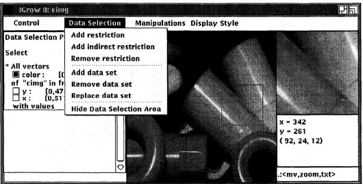
As discussed in section 1, image interpretation modules often require information from many arrays holding partial results. At program execution and debugging time, the programmer needs to be able to visualize these relationships between the data. Figure 2-3 shows VDI's menu to link arrays. It provides mechanisms to restrict arrays ("Add restriction" and "Add indirect re-striction"), as well as tools to simultaneously show the contents of several arrays ("Add data set"). The following subsections describe these mechanisms.

. . . " ' \ u• • • • • • • • • • • • • __ • • • " . " __ " .., • • • • • • __ • • .., _ __ . _ - .• • • • • • • • • • • • __ _ __ • • • __ . ._ .

,

m

rl1\ll 0:dm~

---~_._---_..

_

..~~--_...--_.._~---_...--~~-~_.._._--._._---_.---_._...-._..~---~-~---~._-

QHilJ

Control

Data Selection P

select

>I<All vectors

II

color: [( of "cimg" in fr

D

y: [0,47

Ox: [0,51' with values

Data Selection

Add restriction

Add indirect restriction

Remove restriction

Add data set Remove data set Replace dataset

x

=

342 Y

=

261 (92,24, 12)

[image:9.615.40.570.374.643.2]

.rcmv.zuom.txt>

2.1.2.1 Direct Restrictions

VDI provides basic mechanisms for specifying restricting relationships between arrays. When the programmer restricts an array by another array, VDI displays the primary array using the following rule: "display pixelp[i,j, ...] of the primary array, if the corresponding pixelr[iJ, ...] in the restricting array lies within the specified value range. Otherwise, display a user-specified replacement value".

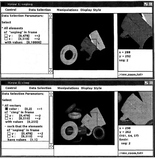
Figure 2-4 shows VDI's restriction mechanism. The upper image in the figure shows a segmen-tation image which contains masks covering three of the eight objects in the scene. The seg-mentation pixels in the masks have values 2 and up, whereas the pixels in the unmasked areas have value 1. The lower image of Figure 2-4 shows how such segmentation information can be linked to the original image. In the data selection menu on the left, the programmer has asked VDI to display all those color pixels of the original image for which the corresponding pixel in the segmentation image is 1, i.e., for which no segmentation mask has yet been constructed. All other pixels are displayed using a replacement value (here: a light gray). Effectively, the seg-mented objects are "masked out of' the original image such that the programmer (as well as the data manipulation modules) can concentrate on the image areas that are not yet interpreted. The masked image shows that parts of the highlights on the objects are not covered by the object masks, and that a small portion of the horizontal (green) cup has been included into the object mask of the diagonal (orange) cup. Similarly, the linking mechanism can be used for analyzing local image properties, such as image gradients or curvature: the original image can be linked to a gradient image, requesting that all pixels with gradients of a specified range be shown.

Currently, VDI only links array elements at the same framing positions in different arrays. If the framing features have different ranges in the arrays, VDI crops the arrays to the common (overlapping) area. A future extension to VDI may provide a transformation mechanism for translating, scaling and rotating coordinates from one array into coordinates in another array. Such mechanisms will be useful for analyzing neighborhood relationships in images (by shift-ing arrays). Automatic scalshift-ing will be essential for analyzshift-ing image pyramids, e.g., for visualiz-ing relationships between pixels at different levels of a pyramid.

[image:11.615.56.554.78.586.2]

···i·G~~w···i·~·;~~lit~;·~l··· ···~n5J]1

..._--- _--- _--- _.- -- _-.-..- _--- - - - _-- --- - .

Control Data Selection Manipulations Display Style

Data Selection Parameters:

Select

... All elements

of "se gimg" in frame

o

y : [0,478] ++2

o

x : [0,510] ++2

with values [0 1 0000]

Data Selection Parameters:

Select

... Allvectors

III color: [0,2] ++1

of "cimgl' in frame

o

y : [0,478] ++2

o

l( : [0,510] ++2

with values [0,255]

- such that the elements of "se gimg" in frame

o

y : [0,478] ++2 Ox: [0,510] ++2

have values [l 1]

Figure 2-4 Direct restrictions on an array

l( =290

Y= 262

(161, 64,57)

Restr: seg:2

2.1.2.2 Indirect Restrictions

In addition to direct restrictions on arrays, VDI accepts indirect restrictions. VDI uses the pixel value p[ij, ...] of the primary array as index into indirectly restricting arrays: "display pixel

p[i,j, ...]of the primary array, if the pixels r[p[ij, ...]] in all indirectly restricting arrays lie in their

specified value ranges. Otherwise, display the specified replacement value".

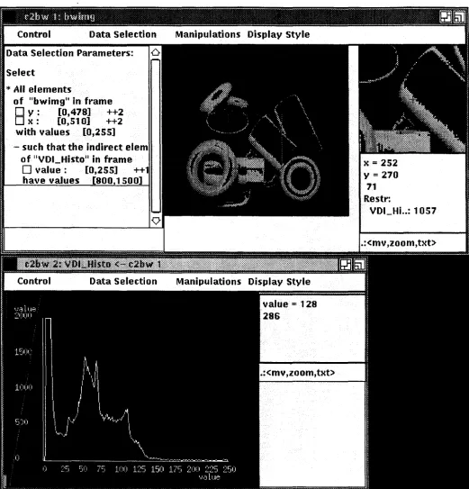
Figure 2-5 demonstrates VDI"s indirect restriction mechanism. For this example, we have con-verted the color image of the plastic scene into a black-and-white image and then generated an intensity histogram - a one-dimensional array of values. The histogram array is shown in the lower half of Figure 2_5.1 2The upper half of the figure displays the intensity image, using the indirect constraint that only pixels be shown whose intensity values occur between 800 and

1500 times in the image.

In general, indirect restrictions can be established between arrays of any dimensions: if the tained feature of the primary array allows for more than one feature value, or if several con-tained features exist, an index vector, pvec(1 ..n)[i,j, ...], has to be used as a multi-dimensional index into a restricting array of appropriate dimensionality. The index vector contains all ele-ments (l ..n)of the cross product of all contained features at the current framing position [ij, ...].

VDI supports dimensional indirect restrictions to a limited extent: it follows the multi-dimensional restrictions of the lowest contained feature. If more than one contained feature ex-ist, all but the lowest one are ignored.

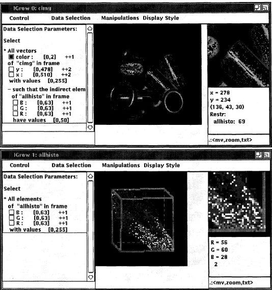
Figure 2-6 shows an example for multi-dimensional indirect linking: we have created a three-dimensional color histogram for the color image of the plastic scene, counting how often each color triple <R,G,B> occurs in the image. The lower half of the figure displays the color histo-gram. To save allocated memory the application program has scaled each color axis down by a factor of 4, such that each color bin now effectively represents 4x4x4 neighboring colors. The application program has informed VDI of this down-scaling operation, and VDI takes it into account in the upper half of Figure 2-6 when it uses the color pixels of the original image as index vectors into the color histogram. In this example, we have requested to visualize all those color pixels in the original image that occur less than 50 times in the histogram. Such pixels are likely to carry a lot of noise, and a vision programmer may be interested in investigating whether there are systematic (i.e., not noisy) patterns. Indeed, the highlights seem to be particu-larly noise-prone, as well as a small area of inter-reflection between the two diagonal cups. Sur-prisingly, one of the small donuts also seems to carry more than the average amount of noise. Of course, this restricting relationship between the color histogram and the original image can-not be a substitute for a real analysis of noise in the image. After all, histograms depend on ob-ject sizes and shapes. However, an interactive and dynamic capability of linking histogramming information to the original image can provide quick intuitions about aspects of computer vision that may need to be considered in the application program.

IThe ID-histogram array is shown as a graph rather than as a row of intensities, because the graph renders the histogramming information (the individual histogram counts) more precisely to the user than the corresponding intensity image. See section 2.2.3 for a discussion of different graphical representations.

Control Data Selection Manipulations Display Style

Data Selection Parameters:

Select

>I< Allelements

of "bwimgllin frame

o

y : [0,47.8.] ++2

OK: [0,510] ++2

with values [0,255]

- such that the indirect elem of "VDLHisto" in frame

o

value: [0,255] ++1 have values [8001500]

x=252 y= 270

71 Restr:

VDLHi..: 1057

.rcmv.znom.txt>

-,···jj1U~itij1~1~$.1%j:~~~~~I~j::l:j~1I@:j:1:~j1:~j~~1:~:n:j::::~::~::1~~~~j~~j~:~1j1~:~j:1~1:::1~1~~~1~1:1~1j1jj~1j~j:~1~j~1~1~~:1~~~1~~~~~::1~~j1:::1jj:1:1:::1jf~j~:::jj1::~i1j::~:~:1:~:1::jj:~:~::jjj~~~j:j~:1:~:::~:::~:::Hj!J

6iJ

Display Style

[image:13.615.44.565.88.631.2]

.:<mv,zoom,txt>

:

_--..

mruw

0; €hUll

~_A_.~ A~__~_.~__~ ...._.._ ~ •• • • • ••__ --..._. ~•••__. ~ ~ _ .__~_~~.

__---Control Data Selection Manipulations Display Style

Data Selection Parameters:

Select

>I< All vectors

III

color: [0,2] ++1 of "cimg" in frame

o

y : [0,478] ++2

ON: [0,510] ++2

with values [0,255]

- such that the indirect elem of "allhisto" in frame

DR: [0,63) ++1

o

G : [0,63) ++1

DR: [0,63] ++1

have values [0 50]

N

=

278

y= 234 (136, 43, 30) Restr:

allhisto: 69

.icmv.zuom.txt>

---~---~---tGrow 1: atlhhto

- - - ~ Control Data Selection Manipulations Display Style

Data Selection Parameters:

Select

>I< All elements

of "allhisto" in frame

DB: [0,63] ++1

o

G : [0,63] ++1

DR: [0,63] ++1

[image:14.617.37.571.80.649.2]

with values [0 255]

Figure 2-6 Indirect multi-dimensional restrictions on an array

-;

----;~b~lfu-;;·;i·~ij·~~~r-···-···-···-····-·-

..

--~-.-

--- --- -- ----.-- --.._._

__.._ _- _.._._ .

~----~-~---_.._-_.~.._---_.-.~.

__

._--_._---~---~---Control Data Selection Manipulations Display style

Data Selection Parameters:

Select

*

All elements

of "original" in frame

D

v :

[0,478] ++2

D

x :

[0,510] ++2 with values [0,255]

*

All elements

of "edge_strength" in fram

D

y : [0,478] ++2

Ox:

[0,510] ++2

with values [0 255]

Control Data Selection Manipulations Display Style

Data Selection Parameters:

Select

*

All elements

of "edge_strength" in fram

D

y : [0,478] ++2

[image:15.617.44.567.76.621.2]

D

x :

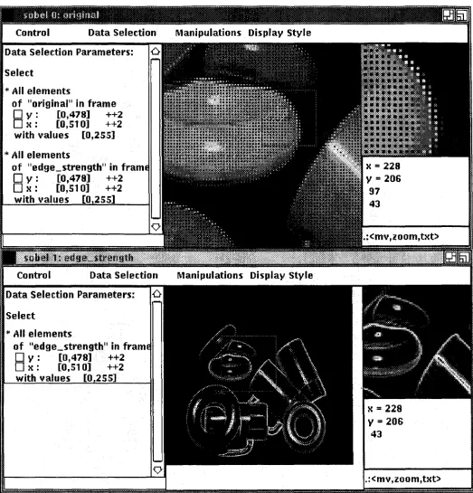
[0,510] ++2 with values [0 255]

Figure 2·7 Links betweenarrays

2.1.2.3 Displaying several linked arrays together

Besides imposing restrictions on the display criteria of a primary array, programmers also need to be able to view several images together. They may either want to see them side by side, with cursors on all arrays moving jointly, or they may prefer seeing all arrays overlaid in a single frame. Preferences will depend on the array contents, the preferred graphical representation, and the amount of detail under consideration. For example, vision researchers have in the past overlaid image flow fields as vector fields on original images, or printed data values (pixels, flow vectors, etc.) on top of (largely zoomed) images.

VDI's data selection area provides the tools to specify such overlay requests interactively. Fig-ure 2-7 shows an example of simultaneously displaying the plastic scene and an edge image generated by the Sobel edge operator. The lower half of the figure shows the edge image. In the upper half, VDI displays all pixels of the original image, as well as all pixels of the edge image. In the selected display style, both images are shown as intensity images. They are overlaid by using a 2x2 pixel area per array element. Within this area, the pixel from the second (edge) im-age is allocated in the upper right bin. The remaining three bins show the pixel value of the first (original) image.' Section 2.2 discusses in more detail which different overlay mechanisms could be used under various circumstances, and which ones are realized within VDI.

2.2 Data Display

VDI provides several mechanisms for displaying arrays. Our central interactive tool is a VDI-window. The programmer can interactively open and close a large number of VDI-windows to view any of the arrays of the application program.

2.2.1 ArrangementofInformation ina VDI-Window

Figures 2-2 through 2-7 have shown typical VDI-windows: The center area displays the array.

Ifthe array is larger than the display area, the programmer can scroll the display area with the left mouse button across the array. As described in section 2.1, the area to the left maintains the current slicing, cropping, subsampling and array linking specifications. A small area in the up-per right contains a zoomed view of a subregion of the array. The programmer can interactively scroll the zoomed subregion with the middle mouse button across the array. The subregion is indicated in the center display area by a red square. The data element at the center of the zoomed region (indicated by a cross) is also presented in printed form in the area underneath the zoomed subregion. The printout shows the position of the element on the framing feature axes (e.g., its

x,y

position), as well as its values along the first contained feature axis (e.g., its red, green and blue color values). Numbers in the following lines represent the related data val-ues in linked or restricting arrays. The programmer can arbitrarily modify this printout in the application program by supplying a specialized printing routine to display any arrangement of pixel-related information in this window.

2.2.2 Interpretations of Mouse Buttons

Depending on the context, VDI interprets the mouse buttons in various ways. The user can in-teractively select a context by pressing "Ctrl" and one of the keys described in the table below. VDI displays the current context in the lower right corner of each VDI-window.

<Ctrl>x <mv.zoom.txt> standard

<Ctrl>t <mouse.txt.i> homogeneous rotations of 3D data

<Ctrl>s <sel,stop,i> select subarea of the image (crop)

<Ctrl>u <...,...,...> user-defined procedure

Section 2.2.1 has described. the standard interpretation of mouse buttons, with the left button triggering a scrolling operation on the large display area, the center button controlling the posi-tioning of data in the small, zoomed area, and the right button causing a data display window with printed pixel values to pop up (see section 2.2.3.3). VDI-windows initially operate under this mouse interpretation until the programmer changes it interactively. The default can be rein-stalled by pressing "<Ctrb-x".

The programmer can rotate three-dimensional displays by selecting the "<Ctrl>t" mouse inter-pretation. The display then rotates while the programmer presses the left mouse button and drags it. If the center button is pressed, a text window pops up, asking the user to specify a rota-tion axis and a rotarota-tion angle. The right button resets the display to the initial posirota-tion.

Window cropping under mouse control can be activated via the "<Ctrlc-s" mouse interpretation. When the left mouse button is pressed, one corner of the rectangle is positioned. The opposite comer then follows the dragging mouse, receiving its final value when the button is released. If the center button is pressed in addition to the left button, the cropping procedure is aborted. The right button resets the cropping parameters to show the entire image.

2.2.3 Graphical Representationsof Arrays

Depending on the application and on the current debugging purpose, programmers need to view their arrays in different graphical representations. To gain a global impression of the data, they may want to look at an intensity-based rendering of the data. Under other circumstances, it may be important to get a closer look at the data in specific areas of interest (see Figure 2-5). Such detail may be more easily conveyed through graphs. In some cases, programmers will even want to see the actual numbers of the data values in a selected region.

In VOl, the programmer can interactively request to view array data as intensities, graphs (ter-rain maps) or printed numbers. Other representations, such as needle maps, have also proven to be useful. Furthermore, interesting research on using audio output and specially designed icons with variable properties (e.g., variable lengths and angles of line segments) is under way[Grinstein et al. 89, Smith and Williams 89]. VOl is a framework through which such dis-play mechanisms can easily be made available to vision programmers. We plan to integrate more representations in the future. We may also provide a mechanism for programmers to reg-ister their own, application-specific display routines with their arrays in the application program such that they can interactively switch into such specialized display modes.

One important issue in displaying arrays in the various graphical representations is the question of dimensionality. How many framing features and how many contained features can be repre-sented adequately as intensities, graphs or printed numbers? The graphical representations are limited in how many framing features they can display at the same time. VOl generally sup-ports one-, two- and three-dimensional display facilities, allowing the programmer to interac-tively rotate three-dimensional renderings. If the programmer specifies higher-dimensional framing criteria, VOl defaults to the n lowest lowest framing features, that can be presented. Other considerations apply to the contained features. The graphical representation, the display hardware and the contained feature type determine how many contained array elements can be shown per framing position. The semantics of VOl's data selection menu request in most gen-eral terms, that the cross product of all contained feature vectors be shown simultaneously for all linked arrays, with the programmer being responsible for cropping the volume of displayable information to a reasonable size. Such needs can be satisfied to different degrees in the different graphical representations. If VOl cannot show all data, it defaults to the lowest n contained fea-tures that it can display.

The following subsections discuss the exact limitations on framing and contained features for intensities, graphs and printed numbers.

2.2.3.1 Intensity-based displays

Intensity-based capabilities for displaying more than one contained feature value are rather re-stricted. A few specialized techniques for displaying particular kinds of contained feature vec-tors have emerged in past years, such as color images (with the contained feature being a color vector of three elements), movie loops (with the contained feature being a time vector or a z-axis) [VoxelView 89], and blink mechanisms (for contained feature vectors of two elements) for which the system alternates between displaying a front and a back buffer [Carlbom et al 91]. Some systems also have a special mechanism to display stereo images. Many of these tech-niques are by now supported by special hardware. VDI exploits existing color display capabili-ties, analyzing the descriptions of feature vectors supplied by the programmer (or extracted from the file name) when the array is created. Accordingly, VDI switches from a black-and-white color map to a colored one, if the contained feature vector under consideration is a color vector, and if the vector has not been cropped to show only one or two color bands. VDI does not yet support stereo display capabilities and automatic blinking. However, as an aid to view a sequence of frames, VDI does provide an interactive mechanism similar to a movie loop to step along a contained feature axis. The mechanism provides a slider with which the programmer can select frames in arbitrary sequence. These capabilities will be extended as necessary.

In addition to providing specialized display mechanisms for specific kinds of contained feature vectors, we need some general mechanisms for viewing arbitrary contained feature vectors. Several windows with linked cursors could be positioned side by side, each showing one par-ticular slice through the data volume. Alternatively, several contained values at a parpar-ticular framing position can be interlaced such that each framing position displays all contained values in a small, local area (see section 2.1.2.3 and Figure 2-7 for an example). Currently, VDI pro-vides an interlacing mechanism to overlay several linked images. For every single array, how-ever, it displays only one contained value (or color triple) per framing position (taken from the lowest index of the lowest contained feature). VDI does not yet support cursor linking to dis-play several linked images side by side. The programmer can, of course, disdis-play several arrays independently in different VDI-windows, as shown in Figures 2-4 through 2-7. But the cursors have to be positioned individually. We plan to provide a cursor linking capability in the future, along with an interactive mechanism to switch between interlacing and cursor linking. In the most general terms, VDI will need to provide interactive tools for the programmer to specify sets of contained features or linked arrays that need to be interlaced, with each set being shown in a separate window. The programmer should also be able to specify interactively, if particular array links or feature vectors should be attached to special-purpose display mechanisms, such as movie loops, blinking mechanisms or color displays. For example, Figure 2-7 might benefit from showing the original image in red and the overlaid edge image in green.

2.2.3.2 Graphs (terrain maps)

As an alternative to viewing arrays as intensity-based displays, programmers may sometimes want to visualize their data as graphs or terrain maps. This graphical representation is more suit-able to conveying detailed information from a small area of the array, whereas the intensity dis-play provides a more global overview.

surface (a terrain map). In this case the two horizontal axes represent the framing features, and the vertical axis represents the element values. The programmer can interactively move and ro-tate terrain maps.

Contained features underlie less restrictions in terrain maps than they did in intensity-based dis-plays: terrain maps of many contained feature values can be shown simultaneously in a single display. VDI supports the display of several terrain maps in a VDI-window. So far, VDI gener-ates terrain maps for all feature values of the lowest contained feature, from all linked arrays. We plan to extend this facility towards displaying several contained features in the future.

Figure 2-8 shows a small area of the color image as a set of terrain maps (center window) and as graphs (lowest window). In this graphical representation, each color band is shown as a sepa-rate terrain map or graph. On the screen, the maps are usually shown in different colors, red, green and blue. The maps show a small area on a green cup in the image. In the segmentation image in Figure 2-4, this area had falsely been assigned to the diagonal (orange) cup above. The terrain maps help us understand the problem: The low plateau in the front part of the terrain maps corresponds to the (very dark) planar facet on the green cup that was falsely segmented into a region with the orange cup. Due to the green object color, the green terrain map has the highest pixel values, while the red and blue color bands should have lower pixel values. The blue terrain map (the lowest one) follows the overall shape of the green map, at lowered intensi-ties. However, the red map (the middle one) behaves rather differently. Instead of dropping into a lower plateau, it actually shows higher values that slowly decrease along the x-axis. The opti-cal phenomenon we are encountering here is inter-reflection of light from the orange cup onto the green cup. This orange light is reflected specularly off the green planar facet into the cam-era, raising the red values disproportionately. Thus, the pixels from this part of the green cup have a much more reddish color than the rest of the cup. The graphs in the lower window show the same phenomenon for a single line along the x-dimension. This is an example of how a pro-grammer can use VOl's interactive debugging capabilities to investigate unexpected results ("problems") when they occur.

2.2.3.3 Printed numbers

Layouts of printed numbers on a screen or on a piece of paper are limited to two dimensions. Thus, no more than two framing features can be shown concisely in this graphical representa-tion. However, if the programmer is willing to scroll back and forth between several related po-sitions in a printout, more than two framing features can be shown as separate blocks of data that are arranged one above the other or next to one another.

Contained feature vectors can be handled the same way: if more than one contained feature value exist, each feature value can be shown in a separate table. This layout style is similar to the cursor-linking mechanism discussed above. Alternatively, contained feature values (as well as any framing feature values in excess of two) can be interlaced. Each table entry then be-comes an n-tuple of information, with nbeing the cross product of all interlaced feature vectors. Clearly, this solution underlies the same layout restrictions as "cursor-linking": more than two dimensions of contained features will be difficult to show within a well-structured layout. Inter-lacing seems to be most useful, when restricted to one dimension, or when it is used to interlace corresponding array elements from several linked arrays.

VDI's current layout strategy exploits the observation that people tend to be interested in only a small data area around a critical point of interest and that entire printouts of large arrays by far exceed the display capabilities of screens and paper. Accordingly, VDI restricts its printout to a small square subarea of the array, centered around the current cursor position. An interactive parameter, "data window size" defines a cropping criterion for all framing features. We do not crop the contained features since the programmer cannot position the cursor with respect to these feature vectors. The programmer can select an area of interest with the cursor by pressing the right mouse button. When an area is selected, VDI pops up a new data display window and prints the values of all array elements in the subarea. The programmer can then study the print-out while keeping an eye on the "overall picture" in the intensity-based display shown sepa-rately. If requested, VDI copies the printed numbers to a file such that the programmer can ob-tain a hardcopy. This practice differs from VDI's mechanism of interactively switching between an intensity-based display and a terrain map. We expect that programmers will gener-ally be interested in checking the array data in several different locations with this mechanism, scrolling the data window across the array by keeping the right mouse button pressed. It would be inconvenient for them to switch graphical representations each time. We may consider pop-ping up a separate window for terrain maps, too, if that proves to be a much-needed shortcut for finding the appropriate small subarray for a terrain map from an intensity-based overview.

In Figure 2-10, only the y-dimension has been selected as a framing feature. Accordingly, the intensity display shows a one-dimensional array (which has been zoomed by a factor of 4). The data printout shows y laid out horizontally, cropped to a data window of size 3. The first con-tained feature,

x,

is printed vertically. It has not been cropped beyond the cropping criteria specified in the data selection menu. The second contained feature, color,is small enough to fit as three separate horizontal tables onto the screen.

V

=

201

(143, 99, 43)

j::::::j~9.!ijl:::g~::::t.:!:mij::::iiPit~j:::::::::::::::::::::::::::::::::::::::::::::::::::::::::::::::::::::::::::::::::::::::::::::::::::::::::I::i:::::,::::::::::::::::::::::::::::::: Control

j:jij:j!~gi:1Qij:j:p~:::j~!jij;ii9:::':::::::::):):)::jj:))::::i::):j:i:i::ji)ii:i!):):,:!:,i!j':iii':i:i:):):;:j:):)::):)::,:j:::):))):):):!:):::':::):)!):))))):):::,:))))::::)):)i::):)::::)j:j::::)::):ij'iiij:):"):::::::j:):)ii,i,}:, Control Data Selection Manipulations Displav St

Select

*

All planes

[II color: [0,2] ++1

[II X : [360,368] ++1

of " cimg" in frame

o

V : [200,208] ++1 .:<mv,2oom,txt>

with values [0255]

Data Selection Parameters:

oolor 0 1 2

Jl [200][201][202] [200] [201] [202] [200][ 201] [202]

x

[360] 142 *143* 145 95 *99* 103 41 *43* 49

(361] 136 *136* 138 90 *93* 95 36 *38* 43

(362] 133 *133* iSS 87 *87* 87 30 *31* 35

[363] 130 *130* 133 82 *82* 85 27 *27* 29

( 3S4] 128 *125* 130 81 *82* 84 25 *26* 27 [365J 130 *130* 130 81 *132* 134 24 *24* 25 [366] 125 *123* 128 78 *79* 81 22 *23* 24 [367] 123 *123* 120 78 *78* 78 22 *22* 23 [368] 123 *120* 120 76 *78* 78 22 *23* 23

0

[image:25.612.143.463.180.618.2]

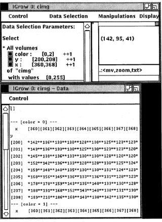
Figure 2-11 shows the color image, with none of the features being selected as framing features. In this case, the frame is reduced to a single element, containing a three-dimensional space of information: Accordingly, the intensity-based display shows a single square which is related to the color triple at the first index of

x

andy. The printed data shows the entire three-dimensional space of contained information. The first contained feature,

x,

is laid out horizontally, the sec-ond one, y, vertically. Since the x-vector contains quite a few (9) elements, three of such tables don't fit horizontally onto the screen/page and the color vector is thus laid out vertically.

Data Selection Parameters:

Select (142, 95, 41)

[color" O}

---x [360)[361][362][363][364][365)[366][367)[368) y

[200] *142**136**133**130**128**130**125**123**123*

[201] *143**136**133**130**125**130**123**123**120*

[202] *145**138**136**133**130**130**128**120**120* (203) *152**142**136**133**128**128*"'130"'*125**124* [204] *159**148**140**135**130**130**131**124**123* (205) *168*... 156*... 145...*136**133...*136**131...*128... 123...

[206) *178**118**159**143**135**140**133**130**128* [207) *188**191... 168...*152...*143... 140...*138 ...*131*... 130...

[208] *189**210**186**168**143**138**142**135**130*

[color

=

I]

---x [360][361)[362}[363][364][365}[366)[367}[368} .icmv.znom.txt>

++1 ++1 ++1

Control

*

All

volumes

[iJ color: [0,2]

[iJ y : [200,208]

[iJ x : [360,368]

of "cimg"

with values [0 255]

(J.![)

[image:26.615.34.581.155.425.2]

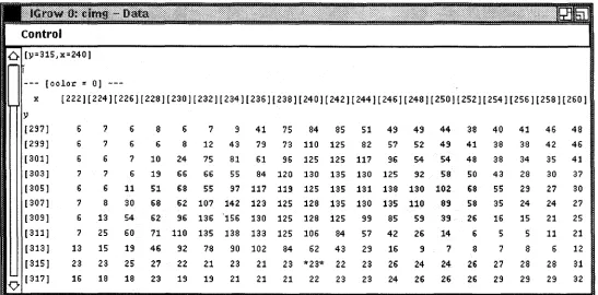
Figure 2-12 picks up on the discussion in section 2.2.3.2concerning inter-reflection from the orange cup onto the green cup. Using a data window size of 20, we now have printed all pixel values (and 'more) that were shown in terrain maps and graphs in Figure 2-8. The figure pre-sents part of the red color band, exhibiting an increase along the x-dimension in the appropriate data area (fory >=315).

control

£} (y=315,x=240]

(colol:

=

OJ

x [222][224J[226][228J[230][232J[234][236](238][240J[242J[244J[246][248][250J[252](254](256][258][260] y

(297] 6 7 6 8 6 7 9 41 75 84 85 51 49 49 44 38 40 41 46 48

(299] 6 7 6 6 8 12 43 79 73 110 125 82 57 52 49 41 38 38 42 46

(301] 6 6 7 10 24 75 81 61 96 125 125 117 96 54 54 48 38 34 35 41

(303J 7 7 6 19 66 66 55 84 120 130 135 130 125 92 58 50 43 28 30 37

(305J 6 6 11 51 68 55 97 117 119 125 135 131 138 130 102 68 55 29 27 30 (307] 7 8 30 68 62 107 142 123 125 128 135 130 135 110 89 58 35 24 24 27 (309] 6 13 54 62 96 136 156 130 125 128 125 99 85 59 39 26 16 15 21 25

(311] 7 25 60 71 110 135 138 133 125 106 84 57 42 26 14 6 5 5 11 21

(313J 13 15 19 46 92 78 90 102 84 62 43 29 16 9 7 8 7 8 6 12

(315] 23 23 25 27 22 21 23 21 23 *23* 22 23 26 24 24 26 27 28 28 31

'0 (317] 16 18 18 23 19 19 21 21 21 22 23 23 24 26 26 26 29 29 29 32

Figure 2-12 Printed numbers for an inter-reflection area in the color image

2.2.3.4 Combinations of several graphical representations

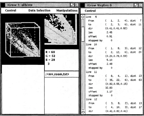
2.2.4 Overlays of symbolic data

In addition to seeing array data, programmers may also want to view symbolic information, overlaid on the images. For example, an image interpretation program might compute a bound-ing box or the center point of a segmented image area, and the programmer might want to dis-play this information on the original image or draw the boundaries of a segmented region. VDI provides basic programming tools for a programmer to write drawing routines and to connect them with VDI. The programmer specifies the drawing commands with respect to the array co-ordinate system. VDI scales, scrolls, rotates and projects the drawings at run-time, according to the interactively selected subsampling, cropping and zooming preferences of the user.

:::f:Jltij:;::::j::~::~II~:I:l.:~J.i::::ii::~:::':::::::::~:::':::::~::::::::::::i::::~::::::::::::::t::~::::::i::::::::::::::,::::::::::::::::::::::::::::::::::::::::

Control Data Selection

-6 line 5

frol'l ( 1, 2, 4), dist 7

to ( 2, 3, 6), dist 11

dir (0.41,0.41,0,82)

len 2.45

offset 0.91

stopped by

o

line 10

frol'l 1, 6, 3), dist 12

to ( 2, 12, 6), dist 20

dir (0.20,0.78,0.59)

len 5.10

offset 2.48

stopped by 0

line 11

.icmv.zoum.txt>

_{froPl ( 6, 4, 1), dist 13}

to ( 35, 22, 6), dist 63

dir (0.82,0.55,0.15)

len 32.83

offset 1.17

stopped by

o

line 12

frol'l ( 3, 8, 2), dist 13

to ( 4, 10, 3), dist 17

[image:27.615.54.553.196.598.2]

0 dir (0.41,0.82,0,41)

Figure 2·13 Graphical overlay of symbolic data on an array

more information about the line segments. For example, line 11 is the long diagonal line run-ning through most of the middle cluster, a yellow color cluster. It contains the pixels of the rightmost diagonal cup in Figure 2-2.

2.2.5 Display Styles

In addition to choosing between several graphical representations, programmers can manipulate the display style in several ways. Figure 2-14 shows VDI's menu for setting and changing vari-ous parameters which influence the display style.

Data Selection Parameters:

Select

... All vectors

[11

color: £0,2] ++1 of "cimg" in frame

D

y : [0,479] ++1

[image:28.615.43.573.192.526.2]

D

x :

[0,511] ++1 with values [0 255]

Figure 2·14 VOl's menu for selecting display styles

large Zoom = 1

large vertical scale =1 large horizontal scale = 1 small Zoom = 2

Data Window Size = 3

ColorMap = Userdef. Colors (Craph) ColorMapWrap= AutoAdjust

Change. ColorMapEntry Initialize current colormap DisplayStyle = Intensities PixelDisplayStyle= oataValue

PixelTransmittance = Opaque (except at 0)

ShowOverlays = True Value Scale= 1.000000 Value Shift = 0.000000 Default Min ReplaceVal

=

0 Default Max ReplaceVal = 0

The first four entries handle different aspects of zooming the large and small array display ar-eas. The large zoom and the large vertical and horizontal scale factors influence the scaling of the large display area. The final vertical scale factor is the product of the zoom factor and the vertical scale. The final horizontal scale factor is computed similarly. Scaling of the small dis-play area is the product of the small zoom factor and the respective large zoom and scale fac-tors. VDI currently zooms by simple pixel replication.

The next four entries are related to different aspects of setting and changing color maps. VDI maintains a large collection of color maps, such as grayscale and color displays, false (pseudo) coloring and random coloring, as well as two maps that can be changed interactively, either via a table of color names or via a graphical interface in which the relationship between pixel val-ues and displayed valval-ues is defined by a red, a green and a blue graph. Each graph is a piece-wise linear function. The programmer can interactively create new knots to break the graphs into smaller linear segments or move or delete existing knots (see Figure 2-15).

o

25 50 75 100 125 150 175 200 225 250

::I\t;,rll:!::i;~\::~:j.fij.i:!t:::!::::::~::\:::::\\:::::::::::::~:~:::::::::::I:::::::::::::::::::::X::\::~:::::':::I:::::~:::::::::\::::I:::::::::::::::::::::::::::\::::':: {::.&¥i{~l~~;::::::··;::::::::;':};·:::: }:::::?::::::\::::n::?~:/:':·::·::.: .:;){::::\\::.::":\:::;:':::..:::::':: :::;.

Control Data Selection Manipulatic commands: <ctr 1>./m/a/dlile/help

[image:29.615.47.572.172.501.2]

move brf.:Qkpoint. 250

Figure 2-15 Graphical Interfaceto change color maps

The tenth entry, "DisplayStyle", lets the programmer switch between an intensity-based graphi-cal representation and a terrain map.

The parameter "PixeIDisplayStyle" specifies whether the displayed colors or intensities are to encode positional information (i.e., the framing position of a data element) or content informa-tion (i.e., the values along the contained feature axes). The opinforma-tion of encoding posiinforma-tional infor-mation can be useful for viewing dimensional sparse arrays (e.g., clusters in high-dimensional feature spaces, such as color histograms) where it is more interesting to see which frame positions are occupied than to know the exact value.

translucency as a function of position (depth along the viewing axis) and/or as a function of the array element values.

VDI's mechanism for graphically overlaying symbolic information on arrays can be turned on and off with the "Show Overlays" button.

The next two entries, "Value Scale" and "Value Shift" specify whether and how to modify the array values before they are displayed, using the formula,

Displayed Value

=

Array Value

*

Value Scale +Value Shift.

This transformation from array values to displayed values is useful for viewing integer or float-ing point arrays which need to be mapped into bytes before befloat-ing displayed.

Finally, the "Default Min Replace Value" and "Default Max Replace Value" parameters are re-lated to the array restriction mechanism (see section 2.1.2). They specify which value will be displayed, if a pixel does not meet all conditions specified in the data selection area. If the pixel is below the acceptable value range, it is replaced by the minimum replacement value. If it is above the range, it is replaced by the maximum replacement value. We plan to extend this mechanism from specifying two parameters to defining a lookup table such that a separate re-placement value for every display value can be set. Such capability can be used for dimming all restricted values or for selectively showing subsets of restricted values in different colors.

2.3 Data Manipulation

VDI provides a few very basic data-manipulation routines, such as file input and output, copy-ing, histogramming and projecting arrays. However, we expect that in most higher-level data interpretation programs, data manipulation is tightly controlled by the application program and that it depends in complex ways on the contents of many related arrays and on the overall state of the data interpretation. For most purposes, we thus expect programmers to write their own manipulation routines and control structures. The programmer can register data manipulation routines with VDI so that the routines can be executed interactively. This provides the mecha-nism for supplying libraries of standard, general-purpose data interpretation routines for interac-tive use. It also opens the door for tentainterac-tive execution of data manipulation routines, such that the programmer can ask questions such as "what would happen, if I applied the following op-eration to my data in the current program state?"

Display Style

HYPOTHESIS DEBUGGING: HYPOTHESIS GENERATION:

-- generate linear hypotheses

· make colorhistogram

· find maxima in diagonal slicesthroughcolorhistogram

· follow maxima through colorhistogram

· backproject histogram

· find connected components - generate illumination hypotheses

· set illumination hypothesis interactively

HYPOTHESIS SELECTION:

- sort linear hypotheses

HYPOTHESIS APPLICATION:

- apply linear/planar hypotheses

linear region growing(1 square seed)

· half-planar region growing(2 square seeds) · region splitting U region)

HYPOTHESIS ARBITRATION:

- separate hypotheses (1 conflict region)

- combine hypotheses(1 conflict region) 6 Write data into file

Step through Data Set (slice)

Project Array

Make Histogram

.~ Make SpecialHistogram Copy this VOl-Widget

Copy current colormap to Default Colormap

Copy current colormap to Default Colormap (BW)

MISC:

- clear overlay

- make histogram of a square image areaU square seed) - make histogram of a region (1 square seed)

select

*

All vectors

iii

color: [0,2J ++1

of "cimg" in frame

o

v :

[0,479J ++1

Ox:

[0,511] ++1

with values [0 255]

3 The Program Interface

The intent in buildingVfrl was to provide programmers with a library of graphical debugging routines that can be included with minimal effort into an application program. It is the goal to keep the program interface as simple and small as possible. Ideally, the VDI-package should be an integral component of a standard debugger or of an integrated programming environment such that it can be called at runtime, without any changes to the application code.

VDI's program interface uses a special data structure, a VDLArrayl, to communicate with ap-plication programs. This data structure contains a pointer to the data, as well as header informa-tion that describes the dimensionality of the array and the ranges and names of the feature axes. VDI provides procedures and macros for initializing, reading in, writing out, copying and ac-cessing VDLArrays.

VDI internally maintains a list of all arrays that an application program registers with VDI. An application program can announce arrays to VDI by either explicitly registering them or by re-questing that they be displayed. In the first case, VDI only enters the array into its list. In the second case, VDI enlists it and also pops up a new VDI-window that displays the array. In either case, the array is thereafter available for interactive viewing, i.e.. the programmer can in-teractively request that it be displayed in a new, pop-up VDI-window or that it be linked to other arrays in already existing windows.

In order for VDI to be a useful debugging tool, it is essential that VDI can be called from any place in the application code and that the application program can continue its computation when the programmer exits from VDI. The most common programming style in X-based win-dowing systems does not support such needs: usually, window-based programs enter an infinite loop, waiting for and dispatching events on an event queue, as initiated through programmer input. Unlike such typical X-based systems, VDI can becalled from an application program as a subroutine, returning control to the application program when the programmer chooses to ter-minate the interactive session with VDI or when VDI runs out of work (its event queue is empty). The application program can specify which of these two exit modes to use when it calls VDI. We also provide an interrupt mechanism via which an application program can test whether the programmer has pressed a special interrupt button to halt the application.

Figure 3-1 shows an example of how programs operate on VDLArrays and how they can inter-act with VDI. The example reads in a two-dimensional image and displays the image in a VDI-window. It registers an array-inversion routine, 'my _ InvertImage2d', with VDI and then calls VDI to start an interactive debugging session. When the user selects the array-inversion routine from the manipulation menu, the module inverts the image, according to the user-specified subsampling, cropping and masking criteria. It periodically (in ProgressIncrements of 10 rows) reports progress to the user by displaying the current contents of the inverted image. The user can interrupt the inversion process to inspect the progress.

#include "VDI.h" VDI_Array Img,Invlmg;

main (argc,argv) int argc; char *argv[];

void my_InvertImage2d(); if (argc < 2) {

printf ("Usage: InvertImage2d <filename>\n"); exit(l);

}

VDl_lnit("Invertlmage2d",&argc,argv); VDl_OpenArray (&Img, argv [1] , "Img") ; VDl_DisplayArray(&Img,NULL);

VDl_ReqisterProcedure("InvertImage2d",my_InvertImage2d,O,O,O,VDI_LOCAL); VDl_Run(VDI_UNTIL_USER_EXIT,VDI_REMOVE_WINDOWS);

}

void my_InvertImage2d(n,ProcType,ControlTag) int n,ProcType,ControlTag;

VDI_Array VDI RestrList int

this_img,restricting_mask; restrictions;

x,xs,xe,xinc,y,ys,ye,yinc,maxval, ProgressIncrement=10,InitVal=UNKNOWN;

VDl_GetWindowHeader (n, &this_img, &restrictions, ''''); if (VDl_Rank(this_img) != 2) (

printf("my_Invertlmage2d: two-dimensional array expected\n"); return () ;

}

VDl_CompileRestrictions

(&this_img,&restricting_mask,&restrictions,VDI AND NFS);

xs VDl_FeatStart(this_img,l); ys VDl_FeatStart(this_img,O); xe VDl_FeatEnd(this_img,l); ye VDl_FeatEnd(this_img,O); xinc VDl_FeatStride(this_img,l); yinc VDl_FeatStride(this_img,O); maxval = VDl_ElemEnd(this_img);

VDl_CopyArrayHeader(&this_img,&Invlmg,"Invlmg"); VDl_AllocArrayData(&InvImg,InitVal);

VDl_Enablelnterrupt("Interrupt Img Inversion"); for (y=ys; y<=ye; y+=yinc) {

for (x=xs; x<=xe; x+=xinc)

if (VDl_ucElement2D(restricting_mask,x,y)) VDl ucPutElement2D

(InvImg,x,y,maxval-VDl_ucElement2D(this_img,x,y); VDI_ShowProqress(InvImg,y,ProgressIncrement,NULL);

if (VDI_Interrupt(» VDI_Run(VDI_UNTIL_USER_EXIT,VDI_KEEP_WINDOWS);

}

4 Other Applications for VDI

[image:34.613.38.571.249.531.2]

VDI is a very general toolkit that can be useful in many application areas other than image in-terpretation. Any application using multi-dimensional arrays can benefit immediately from us-ing VDI, simply by callus-ing the VDI library durus-ing an interactive session with a debugger, such as Saber-C, or by using VDI from inside the program or at the shell-level by using a simple program, "show_array". VDI may be especially useful for analyzing and debugging programs that run on massively parallel (SIMD) machines. Beyond applications that are already using multi-dimensional arrays, many applications exist that do not traditionally present their results in array form, although the data can easily be converted to arrays. For example, many software development tools exist which gather statistical data on the performance of programs, indicat-ing where programs are spendindicat-ing/wastindicat-ing their time. To demonstrate VDI's general usefulness, we have converted such trace data from two software tools into array form .

...,.,-.,... --- ---- - - ----.,-- _-- ~- - - ., - - - ---.,--- ---~---- --- - - - --_ _..,.,--.,- -..,...,- - - --... --- -- -- - -- -- - -...

. ShOWPRt"l...'iS lJ~ H.u~R&l::Utu!!>

~ ~ ~ ~

Control Data Selection Manipulations Display Style Data Selection Parameters:

Select

'" All elements

of

"raskstatus"

in frame

D

task id : [0,44] ++1

D

time: [0,190] ++1

with values [0,13]

- such that the elements of "CPU" in frame

D

task id : [0,44] ++1

D

time: [0,190] ++1

have values [0 8]

time = 85

task id= 11

running Restr:

CPU: 1

.rcmv.zunm.txt>

Figure 4-1 VOl as a tool for visualizing constraints between parallel processes on a MIMO-machine

Figure 4-1 shows a program trace of a program executing as several parallel processes (tasks) on a MIMD-machine [Halstead and Kranz 90], displayed in a VDI-window. The course of time is laid out horizontally, while the vertical axis shows different tasks. The array itself, called "TaskStatus", shows when the tasks are created, run, blocked and terminated during program execution. The overlaid vertical lines illustrate several kinds of dependencies between the tasks.' A second array, "CPU" of the same dimensions states which task runs on which proces-sor at any given point in time. This array can be used to restrict the TaskStatus array such that

the programmer can focus on scheduling patterns observed on subsets of processors. The small, zoomed display area and the text area underneath indicate that task 11 is running on processor 1 at time 85, creating process 12.

I line I bytes I cycles I %I CUfYI %

---+---+---+---+---+---+---0 Main (sobel..c) 103 172 10482540 27.35 27.35

1 Main (sobel,c) 100 200 5866989 15.31 42.66

2 riJain (sobel.c) 99 56 3412920 8.91 51.57

3 Main (sobal ,c) 98 56 3412920 8.91 60.47

4 Main (sobel. c) 102 52 3169140 8.27 68.74

5 nain (sobel. c) 96 52 3169140 8.27 77.01

6 riJain (sobel. c) 101 48 2925360 7.63 84.64

7 Plain (sobel.c) 92 36 2194020 5.72 90.37

8 main (sobel. c) 90 36 2194020 5.72 96.09

9 main (sobel.c) 91 24 1462680 3.82 99.91

:~:~:~:ii.·i

..li.!::.·li!i:I::II:.i:iiiiiiiiiii.i!.lili.:!ilill·I!·!I!I!I!·I·!ii·!li..ii·!i.lii!:ii·.!iiiiiiiill·iiil·liii:lilil.iili.!:iii·i.i·i·iiiliiiiiiii!!liIIK = 28

iii]

line = 100

':,:,:,:,:,:::,:':,:,:,::1:,:,:"1 pline

=

1: 15.31%

[image:35.612.63.549.98.600.2]

renormalized to 55%

lyze an entire program segment. We have devised a simple program, "showprof" which com-piles performance statistics into array form. In principle, the information can be stored as a one-dimensional vector, with line numbers as index. However, to ease overlaying the program text on the profile data, we are using a two-dimensional array. The vertical axis shows increasing line numbers. The horizontal axis presents no added information; the original performance data just is replicated a number of times. The lower window in Figure 2-7 shows the array after ap-propriate zooming. Different percentages are shown as different shades of gray.' The text win-dow to the right indicates that the program spent about 15% of its time in line 100. This is the second highest percentage, covering about 55% of time when compared to the busiest line.

5 Summary

This paper points out that higher-level image understanding systems are lacking adequate de-bugging tools that pay attention to the needs for visualizing many highly inter-related multi-dimensional arrays of data. We suggest to merge graphics programming with debugging tech-nology. To provide general-purpose graphical display routines for multi-dimensional arrays, some common display practices have to be extended. This paper discusses such generalizations and presents VDI as an example implementation. We describe operations on multi-dimensional arrays as composed of three steps, each of which imposes different kinds of requirements on an interactive data visualization tool: .

• Data Selection

When inspecting arrays, a programmer needs to be able to concentrate on subarrays. This requires interactive cropping, subsampling, and thresholding mechanisms, as well as meth-ods to select displayable slices through high-dimensional arrays. The programmer must also be able to inspect arrays in relationship to data in other arrays, if operations on one array depend on data values in the other arrays.

• Data Display

Many representations for displaying arrays of data have been used in various application ar-eas, such as graphs, intensity images and arrays of printed numbers. It depends on the cur-rent focus of the data inspection process which representation is the most suitable. A general-purpose display system needs to provide several such representations and offer tools to the programmer to interactively switch between them.

• Data Manipulation

Besides inspecting the current array contents, a programmer may also wish to interactively test the effect of certain modules of his own on the current data interpretation state. Visual programming is a powerful paradigm for interactively exploring such questions. Within a debugging framework, the programmer should have the option to either keep such investi-gation tentative or to assign the results to the array variables in the program, thus having permanent effect on the further execution of the application program.

So far VDI is only a first, crude step in the direction of providing a visual debugging environ-ment to vision programmers. More needs to be done: VOl is not yet an integral part of a debugger, it can only be called as a display library from a debugger. We also plan to add more data manipulation capabilities to VDI: using a visual programming style, the programmer should be able to execute programmer- and VDI-provided procedures on arrays, with temporary or permanent effect on the array variables. Further extensions to the current framework include adding interactively specifiable transformations between positions in different arrays, providing more extensive programmer customization capabilities, and having VDI run in parallel to the application in a multi-threaded environment or on a separate processor across a network.

The concept of extending debuggers or programming environments with a graphical component for displaying multi-dimensional arrays promises to be a valuable visualization tool for many applications. General-purpose programming languages have seen the use of multi-dimensional arrays over a large range of applications. Among such applications are, of course, the typical image-oriented areas, such as computer vision, computer graphics and image processing. But applications in other areas also often operate on multi-dimensional arrays, such as operations research, scientific visualization, pattern recognition and, in general, numerical or statistical data analysis packages. Furthermore, results in other areas, such as simulation, may be restruc-tured into array form. For example, research on the efficiency of parallel programming mecha-nisms (or systems monitoring computation load on a computer network) could visualize simula-tion results in array form, with one dimension representing time, another one the different processors, a third one different strategies for spreading the work across the processors, with the array content showing the load level at the processors at a given instant in time under a given strategy. Instead of writing many, special-purpose visualization routines for every such applica-tion area, the debugger or programming environment offers the chance to unify efforts across applications.

Acknowledgments