ISSN: 1992-8645 www.jatit.org E-ISSN: 1817-3195
ADAPTIVE SENSING RANGE FOR CO-OPERATIVE
SENSING COGNITIVE RADIO.
1AARTI MANDAL, 2A. KARTHIKEYAN, 3T.SHANKAR, 4V.SRIVIDHYA
1
M.TECH II YEAR Student, School of Electronics Engineering (SENSE), VIT University, Vellore. 2,3Asst. Prof.(Sr.), School of Electronics Engineering (SENSE),VIT University, Vellore.
4Assistant Professor, Kingston Engineering College Anna University Chennai,.
Email: [email protected] ,[email protected], [email protected] 4
ABSTRACT
Cognitive radio is emerging as an effective solution against the spectrum scarcity issue. The main processes which make up the cognitive radio working are the spectrum sensing, learning and adapting procedures. Co-operative sensing is a method in which the nodes share the spectrum sensed data. In ad-hoc network the decentralized nature makes it quite difficult to gather sensing data with constraints like energy consumption, shadowing, hidden terminal and fading effect. In cognitive radio ad-hoc network these effects creates issues in spectrum allocation and management. In this paper, the hidden terminal issue is considered with the solution of adaptive sensing range in a static network. The nodes in the ad-hoc network have sensing and transmitting ranges. The sensing helps to gain knowledge about the channels which are occupied by overhearing the RTS/CTS or ACK transmission or reception by the nearby nodes. The sensing range of a node is always greater than the transmitting range of a terminal. The sensing range if varied as per the transmission to the receiver then hidden node issue can be dealt to a great level. With the help Cognitive radio Network Simulator (CR-NS) adaptive sensing is simulated for an ad-hoc network and also its effect on throughput, packet loss, normalized routing load, end-to-end packet delay is also compared with respected to a fixed sensing environment.
Keywords: Cognitive Radio, Hidden Node, Co-Operative Sensing, Cognitive Radio Network Simulator
(CR-NS).
1. INTRODUCTION
Present day telecommunication scenario is such that the spectrum resource is proving to be insufficient and thereby effective method for higher utilization of available resources needs to be developed. Cognitive radio is theoretically proving to emerge as a good solution. The idea of cognitive radio was first given by J. Mitola in 2002[1]. The fundamental task of a cognitive radio (CR) is to locate a free channel in the CR network and adapt to its characteristics for its usage. In this task a major step is spectrum sensing. A cognitive radio network is a secondary network over a primary network.
Later to sensing process comes the learning and adapting process. The learning and adapting process include genetic algorithm (GA), neural network (NN), Hidden Markov Model (HMM) method and Fuzzy logic method.
Spectrum sensing in cognitive radio network:[2]
Spectrum sensing is a method by which the radio locates the white spaces (free spectrum slots) by avoiding any interference to the primary user (PU) and the other secondary user (SU) in the network. An individual node can perform spectrum sensing by various sensing methods as mentioned below:
1. Energy detection: the secondary user (SU) maintains a threshold over which it decides the presence of the primary user (PU) in a channel.
ISSN: 1992-8645 www.jatit.org E-ISSN: 1817-3195 Other methods are Hough’s transform, Eigen
value method, time-frequency method etc. however, in a network if the nodes instead of performing individual processes co-operate to share the sensed data among themselves will reduce the burden on the nodes and help in efficient performance.
Problems faced by nodes in the practical environment:
Hidden node problem:
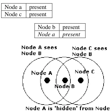
[image:2.612.101.287.311.498.2]Consider three nodes, node A,B and C as shown in figure1.
Figure 1: Hidden Node Problem
The node A can sense the presence of node B as it lies within the range of A. Similarly, node B can sense node C and vice-versa. However, node C cannot sense node A as it lies outside its range. Thereby, node A and node C are said to be hidden from each other. It can happen that node A and node C might send data simultaneously to node B leading to collision and loss of packets and also multiple re-transmissions from both ends to gain access to the channel, thus leading to inefficient network. In cognitive radio, the hidden node problem can occur when a SU is in the range of the primary receiver but absent in the range of the primary transmitter. Thus, when SU and primary transmitter transmit data to primary receiver, collision will occur.
Fading and Shadowing effect:[3]
Shadowing is caused when a node lies in the shadow of a big obstacle and becomes undetectable by the other nodes. In some situation the signal level i.e. the power level of the signal gets reduced drastically thus making it undetectable.
Shadowing effect extend for 10’s to 1000’s of wavelengths and increases for outdoor environment, thus it is expected to be a major factor for limiting sensing operations.
Methods to avoid shadowing effect includes technique to detect users with low SNR (i.e. -20dB 0r lower) [3], sensing of nodes even when a receiver is in shadow. However, these methods have disadvantages of long observation time for spectral occupancy. Other method which is gaining attention is the use of collaborative sensing. [4]
The method wherein nodes share the sensed data is called as co-operative sensing.
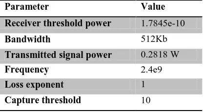
2. CO-OPERATIVE SENSING[5]
Node b present
[image:2.612.327.514.381.604.2]Node c present
Figure 2: Co-Operative Sensing
In co-operative sensing the node A and node C came to know about each other’s existence because of the sharing of information from node B. The sensing is performed first individually and then sharing takes place. However, if a node C would have adaptive sensing range then C would have detected the presence of A and also Node a present
Node c present
Node b present
ISSN: 1992-8645 www.jatit.org E-ISSN: 1817-3195 nodes ahead it if the physical properties like the
power level permits it to do so.
The nodes taking part in co-operative sensing has different ranges namely, transmitting/ receiving range and carrier sensing range. The transmitting/ receiving range is the range upto which the nodes can transmit/receive data to other node. The carrier sensing range is the range upto which a node can detect the presence of another node. The sensing range can help in avoiding the interference from other users. It is always kept larger than transmitting range.
Advantages in co-operative sensing method is as follows:
1. Hidden node problem is reduced as compared to individual sensing : Individual spectrum sensing has higher chances of hidden node problem due to non-cooperative nature and range limitation. This effect is thus reduced to some extent in co-operative sensing as the nodes will have knowledge of the nodes present in their neighbor’s neighbor which mainly remain hidden in other case.
2. Increase in agility and accuracy: the cooperation among the nodes provide more accurate picture of the network to the nodes and also improves the channel move decision thereby, increasing the agility. The improved accuracy also improves the reliability over the network.
3. Reduced false alarms: False alarms are caused in cognitive network when a SU makes a wrong decision about channel occupancy by the PU or other SU. Since this case is less likely in co-operatively sensed network, false alarms are reduced.
However, in some situation when a receiving node is close to the transmitting node, to avoid interference from other nodes the sensing range need not be of larger radius. This can also help the energy conserved to be utilized to increase the carrier sensing range when a receiving node is at far distance. This paper works towards studying the throughput, packet loss between nodes performing adaptive sensing range to
combat hidden node problem using IEEE 802.11 MAC in a cognitive radio ad-hoc network. The simulation is performed in NS-2.31 (CR-NS) environment.
3. ADAPTIVE SENSING RANGE
METHOD
Consider a large scale path loss model with the assumption that all the nodes have the same transmission power and other radio parameters. The assumption is made to simplify the calculation. The received power at distance d is given by:
𝑃𝑟=𝐺𝑡𝐺𝑟𝑃𝑡 ℎ𝑡2𝑑ℎ𝑟∝ 2
where Pt is the transmitted power, ht and hr are the heights of the transmitter and receiver antennas respectively, Gt and Gr are the antenna gains, d is the distance between the transmitter and the receiver. α is the path loss exponent which reflects how fast the signal attenuates. (e.g., 4 in the two-ray ground reflection model and 2 in a free space model).
If Pr and Pi denotes the power received at the receiver and power received at the interfering node which are at a distance d and r respectively from the transmitter, then the signal to the interference ratio, neglecting the thermal noise, is given by[6],
𝑆𝐼𝑅=𝑃𝑟𝑃𝑡=𝐺𝑡𝐺𝑟𝑃𝑡
ℎ𝑡2ℎ𝑟2
𝑑∝
𝐺𝑡𝐺𝑟𝑃𝑡 ℎ𝑡2𝑟ℎ𝑟∝ 2
=�𝑑�𝑟 ∝
For the correct reception, SIR > = S0
which means for the interfering node must be at least
�𝑆0
∝ ×𝑑 meters from the receiver.
Interference range Ri is given by[4],
𝑅𝑖=∝√𝑆𝑜 ×𝑑
The transmitting range(Rt) and sensing range (Rs) is given by,
𝑅𝑡=𝑑̅ �𝑃����𝑃𝑟�𝑟𝑥 1 ∝
where Prx is the reference signal strength as measured at the distance d
ISSN: 1992-8645 www.jatit.org E-ISSN: 1817-3195
𝑅𝑠=𝑑̅ �𝑃����𝑃𝑐�𝑟𝑥 1 ∝
where Pc denotes the carrier sensing threshold.
The sensing range of the SU transmitter must be upto the transmitter for a hidden receiver node which can be a PU or other SU. Thus, the minimum sensing range is[6],
𝑅𝑠=𝑑̅ �𝑃����𝑃𝑐�𝑟𝑥 1 ∝
=𝑅𝑖 +𝑅𝑡= (1 +∝√𝑆𝑜) ×𝑅𝑡
The neighboring nodes can correlated their location ri from the hidden node based on the received power of the request packet send,
𝑟𝑖= �𝐺𝑡𝐺𝑟ℎ𝑡2ℎ𝑟2𝑃𝑡𝑃𝑟
∝
=𝑘 × �1
𝑃𝑟
∝
Where, k=∝√𝐺𝑡𝐺𝑟ℎ𝑡2ℎ𝑟2𝑃𝑡 is constant.
Thus the cooperative sensing range (CPSR) is given by[7],
𝐶𝑃𝑆𝑅=𝑅𝑠 − 𝑟𝑖=��1 +∝√𝑆𝑜�×𝑅𝑡�
− �𝑘 × �1
𝑃𝑟
∝
�
4. SIMULATION ENVIRONMENT AND
CALCULATION
For the verification of the theory NS-2.31[8,9] is used as the simulation tool. NS-2.31 has features available for implementing cognitive radio scenario with the Cognitive Radio Network Simulator (CRNS) freely available as an open source. [10]
The CRNS performs energy detection method and shares the data with the neighboring nodes.
The network setup considered for verification is as follows.
0 9 3 8 4 1 7 2 6 5
Figure 3: Node Arrangement
The parameter setup for the network are:
Parameter Value
Channel Wireless
Propagation model Shadowing
Physical layer Wireless
Antenna type Omni-directional
Routing protocol AODV
Queue type Priority queue
Maximum number of packet in queue
50
MAC layer type 802.11
Number of nodes 10
Simulation time 50
Table 1: Parameter set in NS-2.31 with CR-NS
Two situations are considered for comparison: first with fixed sensing range of 550m i.e. threshold of 9.21756e-11 and the other with adaptive sensing range. Also a small amount of mobility was set for the nodes.
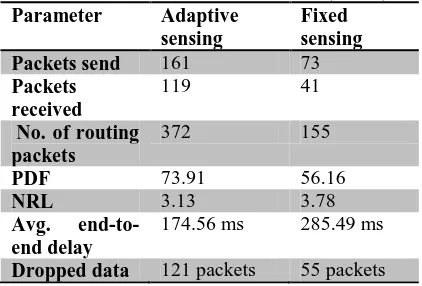
[image:4.612.319.528.450.565.2]The nodes were setup with:
Table 2: Parameter Set For Each Node
Parameter Value
Receiver threshold power 1.7845e-10
Bandwidth 512Kb
Transmitted signal power 0.2818 W
Frequency 2.4e9
Loss exponent 1
Capture threshold 10
.
TCP traffic pattern was: node 5 to node 6, node 2, node 7, node 1, and node 4.Later, node 6 to node 7.
Calculation of sensing range for node 5 for transfer of TCP packet to node 6:
Pt = 0.2818 W default for NS-2.31 Gt = Gr = 1 default for NS-2.31 ht = hr = 1.5m default for NS-2.31 d = 300 m calculated
ISSN: 1992-8645 www.jatit.org E-ISSN: 1817-3195
Thus, 𝑃𝑟=�0.2818 ×1×1×1.52×1.52�
(8.1×10⁹) = 176.125 ×
10−12
𝑘= �4 (1 × 1 × 1.52× 1.52× 0.2818= 1.093
𝐶𝑃𝑆𝑅=��1 +4√10�× 250� − �1.093 ×
�176.1251×10⁻¹² 4
�= 394.57 m
Parameters considered for verification within the network are:
Throughput: is average rate of successful message delivery over the communication channel.
𝑡ℎ𝑟𝑜𝑢𝑔ℎ𝑝𝑢𝑡
=�
𝑛𝑜.𝑜𝑓𝑝𝑎𝑐𝑘𝑒𝑡𝑠𝑠𝑒𝑛𝑑𝑓𝑟𝑜𝑚𝑎𝑛𝑜𝑑𝑒𝑡𝑜𝑜𝑡ℎ𝑒𝑟𝑛𝑜𝑑𝑒
𝑤𝑖𝑡ℎ𝑠𝑎𝑚𝑒𝑠𝑒𝑞𝑢𝑒𝑛𝑐𝑒𝑛𝑢𝑚𝑏𝑒𝑟
𝑡𝑜𝑡𝑎𝑙𝑠𝑖𝑚𝑢𝑙𝑎𝑡𝑖𝑜𝑛𝑡𝑖𝑚𝑒 �
Packet loss: number of packets which remain undelivered to the destination node.
𝑃𝑎𝑐𝑘𝑒𝑡𝑙𝑜𝑠𝑠
= (𝑛𝑜.𝑜𝑓𝑝𝑎𝑐𝑘𝑒𝑡𝑠𝑠𝑒𝑛𝑑𝑓𝑟𝑜𝑚𝑎𝑠𝑒𝑛𝑑𝑒𝑟 )
−(𝑛𝑜.𝑜𝑓𝑝𝑎𝑐𝑘𝑒𝑡𝑠𝑟𝑒𝑐𝑒𝑖𝑣𝑒𝑑𝑏𝑦𝑡ℎ𝑒𝑟𝑒𝑐𝑒𝑖𝑣𝑒𝑟 )
Normalized routing load (NRL)[11]: is number of routing packet per data packet delivered at destination.
𝑁𝑅𝐿=�𝑛𝑜.𝑜𝑓𝑟𝑜𝑢𝑡𝑖𝑛𝑔𝑇𝐶𝑃𝑝𝑎𝑐𝑘𝑒𝑡𝑠𝑝𝑎𝑐𝑘𝑒𝑡𝑟𝑒𝑐𝑒𝑖𝑣𝑒𝑑�
Packet delivery fraction (PDF)[11]: is the total number of packets send and received over the whole network.
𝑃𝐷𝐹
=�𝑛𝑜.𝑜𝑓𝑝𝑎𝑐𝑘𝑒𝑡𝑠𝑛𝑜.𝑜𝑓𝑝𝑎𝑐𝑘𝑒𝑡𝑠𝑠𝑒𝑛𝑑𝑜𝑣𝑒𝑟𝑟𝑒𝑐𝑒𝑖𝑣𝑒𝑑𝑡ℎ𝑒𝑛𝑒𝑡𝑤𝑜𝑟𝑘� × 100
Average end-to-end delay[11]: is delay taken by a packet to be send and received in the network.
𝑑𝑒𝑙𝑎𝑦
=�𝑒𝑛𝑑𝑡𝑖𝑚𝑒𝑜𝑓𝑛𝑢𝑚𝑏𝑒𝑟𝑟𝑒𝑐𝑒𝑖𝑣𝑒𝑑𝑜𝑓𝑝𝑎𝑐𝑘𝑒𝑡 − 𝑠𝑡𝑎𝑟𝑡𝑝𝑎𝑐𝑘𝑒𝑡𝑠 𝑡𝑖𝑚𝑒�
Number of packets dropped[12]: the packet send by a node but not received by the receiver.
5. SIMULATION RESULTS
[image:5.612.318.529.313.456.2]The results obtained can be tabulated as:
Table 3: Result Obtained In NS-2.31with (CR-NS)
Parameter Adaptive
sensing
Fixed sensing
Packets send 161 73
Packets received
119 41
No. of routing packets
372 155
PDF 73.91 56.16
NRL 3.13 3.78
Avg. end-to-end delay
174.56 ms 285.49 ms
Dropped data 121 packets 55 packets
ISSN: 1992-8645 www.jatit.org E-ISSN: 1817-3195 thus packets were not send at all to the
destination node.
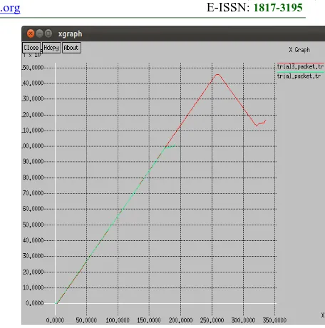
[image:6.612.309.537.76.306.2]The throughput over the network is as shown in figure below. The green line is for the fixed case
and red for the adaptive case. It can be observed that the throughput in adaptive case is quite high as compared to the fixed case.
In figure 5, the packet loss for transmission
between node 5 and node 2 is shown. The red indicates the adaptive and the green indicates the fixed environment. The location of node 5 is 900m and that of node 2 is 400m. When node 2 moved away from node 5 to a distance greater than 550m, node 5 decided that node 2 is absent and did not transfer the packets. However, in case of adaptive sensing, the node 2 was sensed and thus packets were transmitted. When node 2 went beyond the maximum limit if sensing range then the transmission were stopped finally.
Figure 5: Packet Loss Between Node 5 And Node 2.
6. CONCLUSION AND FUTURE WORK
Adaptive sensing method for co-operative sensing has been discussed and its effect on the network characteristics has been observed. The work can be extended by incorporating a learning process like the genetic algorithm, neural network, fuzzy logic so that the cognitive nodes can adapt to the required channel characteristics. Also this adaptive sensing method can be included to develop a MAC layer for the cognitive radio ad-hoc networks.
REFRENCES:
[1] J. Mitola, “Cognitive Radio an Integrated Agent Architecture for Software Defined Radio”, PhD thesis, KTH Royal Institute of Technology, Stockholm, Sweden, 2000. [2
]
Tevfik Y¨ucek and H¨useyin Arslan,”Asurvey of spectrum sensing algorithms for cognitive radio application”, IEEE Communications Surveys & Tutorials, Vol. 11, No. 1, First Quarter 2009
.
[3] Rajesh K. Sharma, Jon W.
Wallace,“Experimental characterization of indoor multiuser shadowing for collaborative cognitive radio”, Antennas and Propagation, 2009. EuCAP 2009. 3rd European Conference.
[image:6.612.84.541.78.459.2][4] Jing Zhang, Zheng Zhou, Haipeng Yao, Lei Shi, Liang Tang, Zhigang Xu, “spectrum
[image:6.612.89.293.209.409.2]ISSN: 1992-8645 www.jatit.org E-ISSN: 1817-3195 sening using collaborative beamforming for
ad-hoc cognitive radio networks”, IEEE ISCIT,2010.
[5] Ian F. Akyildiz, Brandon F. Lo ∗, Ravikumar Balakrishnan, “cooperative spectrum
sensing in cognitive radio network: a survey” ,Physical Communication 4(2011), Elsevier.
[6]
K. Xu, M. Gerla, and S. Bae, “Effectiveness of RTS/CTS
handshake in IEEE 802.11 based Ad Hoc
Networks,” Ad Hoc Networks 1
(ELSEVIER),pp. 107-123, 2003.
[7]
Jongwon Shim, QiCheng , Venkatesh Sarangan,“cooperative sensing with adaptive sensing ranges in cognitive ad-hoc networks,” IEEE conference CROWNCOM,2010.
[8] ns
manual, available at:
http://www.isi.edu/nsnam/ns/ns-documentation.html
[9]ns tutorial at:
http://www.isi.edu/nsnam/ns/
[10]
Online:
http://stuweb.ee.mtu.edu/~ljialian/
[11]
Sabina Baraković, Suad Kasapović, and
Jasmina
Baraković, “
Comparison of MANET Routing Protocols in Different Traffic and Mobility Models”. Available at: http://journal.telfor.rs/published/no3/no03_p02_f in.pdf[12] Kishan Singh Rao, Laxmi Shrivastava, “Efficient Local Route Repair Method in AODV to Reduce Congestion in MANET”, Corona Journal of Science and Technology, Vol. 1, No. 1, October 2012.
[13] Shan Lin, Jingbin Zhang, Gang Zhou, Lin Gu, Tian He, John A. Stankovic, “ATPC: Adaptive Transmission Power Control for Wireless Sensor Networks”. Available at:http://www.cs.virginia.edu/~stankovic/ps files/ATPC.pdf
[14]
Daji Qiao, Sunghyun Choi, Amit Jain, Kang G. Shin, “Transmit Power Control in IEEE 802.11a Wireless LANs” . available at:http://www.staff.ul.ie/bgleeson/docs/vtc03. pdf
[15]
Ian F. Akyildiz *, Won-Yeol Lee, Kaushik R. Chowdhury, “CRAHNs: Cognitive radio ad hoc networks” , Elsevier.Available at:
http://www.eee.metu.edu.tr/~baykal/files/ch ran.pdf