Semantic aware Bayesian network model for actionable knowledge discovery in linked data

S e m a n ti c a w a r e B ay e si a n

n e t w o r k m o d e l fo r a c ti o n a bl e

k n o wl e d g e d i s c ov e r y i n li n k e d

d a t a

Alh a r bi, HYM a n d S a r a e e , M H

h t t p :// dx. d oi.o r g / 1 0 . 1 0 0 7 / 9 7 8-3-3 1 9-4 1 9 2 0-6_ 1 1

T i t l e

S e m a n t i c a w a r e B ay e si a n n e t w o r k m o d el fo r a c ti o n a b l e

k n o wl e d g e d i s c ov e r y in li n k e d d a t a

A u t h o r s

Alh a r bi, HYM a n d S a r a e e , M H

Typ e

C o nf e r e n c e o r Wo r k s h o p I t e m

U RL

T hi s v e r si o n is a v ail a bl e a t :

h t t p :// u sir. s alfo r d . a c . u k /i d/ e p ri n t/ 4 3 0 0 9 /

P u b l i s h e d D a t e

2 0 1 6

U S IR is a d i gi t al c oll e c ti o n of t h e r e s e a r c h o u t p u t of t h e U n iv e r si ty of S alfo r d .

W h e r e c o p y ri g h t p e r m i t s , f ull t e x t m a t e r i al h el d i n t h e r e p o si t o r y is m a d e

f r e ely a v ail a bl e o nli n e a n d c a n b e r e a d , d o w nl o a d e d a n d c o pi e d fo r n o

n-c o m m e r n-ci al p r iv a t e s t u d y o r r e s e a r n-c h p u r p o s e s . Pl e a s e n-c h e n-c k t h e m a n u s n-c ri p t

fo r a n y f u r t h e r c o p y ri g h t r e s t r i c ti o n s .

Semantically Aware Bayesian Network Model for

Actionable Knowledge Discovery in Linked Data

Hasanein Alharbi, Mohamad Saraee

1

School of Computing, Science and Engineering, University of Salford-Manchester, Greater Manchester, England M5 4WT

[email protected],[email protected]

Abstract.The majority of the convential mining algorithms treat the mining process as an isolated data-driven procedure and overlook the semantic of the targeted data. As a result, the generated patterns are abundant and end users cannot act upon them seamlessly. Furthermore, interdisciplinary knowledge could no be obtained from domain-specifi silo of data.

The emergence of Linked Data (LD) as a new model for knowledge representation, which intertwines data with its semantics, has introduced new opportunities for data miners. Accordingly, this paper proposes a Semantic-Aware Bayesian network (BN) model, which exploits the semantic aspectes of the LD structure.It integrates five semantic relations in the mining process.

In contrast to the exisiting mining algorithms, the proposed model do not transform the original format of the LD set. So, it not only accomodates the semantic aspects in LD,but also caters to the need of connecting different data-sets from different domains.

Keywords: Linked Data (LD). Actionable Knowledge Discovery (AKD). Bayesian Network (BN).

1

Introduction

The term Data Mining (DM) refers to methods that aim to extract useful information and knowledge from data. Fayyad et al. have defined these methods as the non-trivial process of identifying valid, novel, potentially useful and ultimately understandable patterns in a database [1,2].

This gap has appeared as a result of two major drawbacks, namely, quantity and quality; the former states that the generated patterns are abundant while the latter indicates that they cannot be integrated seamlessly into the business domain [3], [6]. Upon further investigation, it appears these drawbacks have been caused as a result of viewing the mining process as data driven trial and error practices and ignoring the surrounding knowledge [3], [7]. Consequently, the mining philosophy has faced a paradigm shift from a data-centered to a knowledge-centered process, which aims to integrate the surrounding knowledge such as data intelligence into the mining process [3], [8]. Even though the data intelligence could be represented using various tech-niques, recently LD introduced a new technique to intertwine the data and its seman-tics in one package. Coupling the data with its semanseman-tics not only brings new oppor-tunities for data miners but also raised some challenges; for example, how to identi-fied the interesting transactions in heterogeneous data sets, which has been built based on the description logic and used the triple (subject-predicate-object) format [9,10]. To this end, this paper proposes a semantic-aware Bayesian network model, which exploits the semantic nature of LD and implicitly accommodates the data intelligence in the mining process. The proposed approach consists of the following steps:

1. Convert the original LD file into BN, which preserves the semantics of the LD file. 2. Initializes the Conditional Probability Tables (CPT’s) with default values.

3. Calculate set of probabilistic constraints using the concept of Maximum a Posterior estimation (MAP) in such a way that it reflects the semantic relations between nodes in the constructed BN.

4. Approximate the CPT’s initial values to comply with the set constraints calculated in the second step using the concept of Iterative Proportional Fitting Procedure (IPFP).

The contributions of this paper are twofold. Firstly, the model integrates five semantic relations in the mining process, namely, equivalent to, complement of, disjoint with, intersection of and union of. Secondly, it does not change the original format of LD set and consequently, it caters for the need of linking various data-sets from multidis-ciplinary domains using the design principles of LD. The proposed model tested using five sets of synthesis data and the initial results are promising.

The remainder of this paper is organized as follows: In section 2 the notion of con-verting LD file into BN is explained in detail, while the probabilistic constraints esti-mation methods are illustrated in section 3. IPFP is briefly discussed in the section 4, and section 5 discusses in detail the empirical implementation and the initial results. Finally, the paper is concluded in section 6.

2

Bayesian Network Topology Construction

BayesOWL consists of a set of construction rules, which convert ontology files into BN directed acyclic graphs (DAG), which preserve the semantics of the original on-tology file [11,12]. Likewise, the model proposed in this paper follows the same rules to convert the given LD file into BN DAG.

de-fault values. Then, the integration of the given probabilistic constraints is implement-ed in the second phase [13,14].

The process of construction BN DAG from the given ontology file is governed by a set of rules. The conventions underpinning these rules can be summarized in the fol-lowing points [12], [15]:

1. Every primitive or defined class is mapped into binary variables. 2. Connect each parent superclass with its child subclass by an arc.

3. For each concept class C is defined as the intersection of a set of classes Ci ={ C1,

….., Cn}; a subnet is created in such a way that there is a link from C and each

class in the set Ci toward the class C. Furthermore, there is a link from C and each

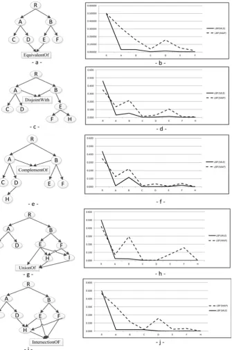
class in the set Ci moves toward a logical node called LNodeIntersection. Figure

1.a depicts the creation of the intersection subnet.

4. For each concept class C is defined as the union of classes Ci ={ C1, ….., Cn}; a

subnet is created in such a way that there is a link from C to each class in the set Ci.

Furthermore, there is a link from C and each class in the set Ci moves toward a

log-ical node called LNodeUnion. Figure 1.b illustrates the creation of the union sub-net.

Fig. 1. LNodeIntersection & LNodeUnion [11]

5. For each two concept classes C1 and C2 are defined as complements of, equivalent

to, disjoint with each other logical nodes (LNodeComplement, LNodeEquivalent, LNodeDisjoint) are created, which take two input links from C1 and C2. Figures

2.a, 2.b and 2.c depict the creation process for LNodeComplement, LNodeEquiva-lent and LNodeDisjoint respectively.

It clearly can be seen that the generated DAG contains two types of nodes, namely, regular nodes, which represent classes and logical nodes, which show the logical rela-tion among classes [11], [15]. The combinarela-tion of these two types of nodes forms the structure of the BN.

The second component of BN is the conditional probability table. As discussed in the previous paragraph, the generated DAG contains two types of nodes, logical and regular. Consequently, the CPT’s for each type should be calculated. The following subsection explains in detail the CPT’s calculation process [11], [16, 15].

2.1 CPT’s calculation for logical nodes

It has been stated that the generated DAG caters for five different types of logical nodes, which are associated with five logical operations in ontology. The CPT for each logical node is determined by its logical relations. The following subsections explain the CPT creation process for each logical node.

CPT creation for Complement of logical relation.

The complement relation between two concepts classes C1 and C2 is true IFF

𝑐𝑐1𝑐𝑐2˅𝑐𝑐1𝑐𝑐2 is true. Table 1 describes the CPT for complement of relation.

CPT creation for Disjoint with logical relation.

The disjoint with relation between two concept classes C1 and C2 is true IFF

𝑐𝑐1𝑐𝑐2˅𝑐𝑐1𝑐𝑐2˅𝑐𝑐1𝑐𝑐2 is true. Table 2 describes the CPT for disjoint with relation.

CPT creation for Equivalent to logical relation.

The equivalent to relation between two concept classes C1 and C2 is true IFF

𝑐𝑐1𝑐𝑐2˅𝑐𝑐1𝑐𝑐2 is true. Table 3 describes the CPT for equivalent of relation.

Table 1. CPT for LnodeComplementOF [11]

Table 2. CPT for LnodeDisjointWith [11]

Table 3. CPT for LnodeEquivalentTo [11]

C1 C2 True False C1 C2 True False C1 C2 True False

T T 0 1 T T 0 1 T T 1 0

T F 1 0 T F 1 0 T F 0 1

F T 1 0 F T 1 0 F T 0 1

F F 0 1 F F 1 0 F F 1 0

CPT creation for Intersection of logical relation.

The class C, which is the intersection of C1 and C2 is true IFF

𝑐𝑐𝑐𝑐1𝑐𝑐2˅𝑐𝑐𝑐𝑐1𝑐𝑐2˅𝑐𝑐𝑐𝑐1𝑐𝑐2˅𝑐𝑐𝑐𝑐1𝑐𝑐2 is true. Table 4 describes the CPT for the intersection of relation.

CPT creation for Union of logical relation.

Table 4. CPT for IntersectionOf [11] Table 5. CPT for UnionOF [11]

C C1 C2 True False C C1 C2 True False

T T T 1 0 T T T 1 0

T T F 0 1 T T F 0 1

T F T 0 1 T F T 1 0

T F F 1 0 T F F 0 1

F T T 0 1 F T T 1 0

F T F 1 0 F T F 0 1

F F T 0 1 F F T 0 1

F F F 1 0 F F F 1 0

2.2 CPT calculation for regular nodes

The CPT‘s for regular nodes are computed by applying the Bayesian theorem as fol-lows. P(C|⫪_c) where C is the class of the regular node and ⫪_c is the set of its parents. The P(C=True |⫪_c) = 0 if any of its parents are false. Hence, the probability for any regular class C is calculated only when all of its parents are in true status. This scenar-io is denoted as P(C|⫪_c+) where ⫪_c+ represents the set of parent classes in true status. This method is used to calculate the probability when probabilistic data is available. Otherwise, a default value (0.5) is assigned based on equation (1) [11], [13].

P (C=True|⫪_𝑐𝑐+) = P(C=False|⫪_𝑐𝑐+) =0.5. (1)

3

Probabilistic Constraints Estimation

The process of converting OWL (i.e. LD) file into BN consists of two phases. In the first phase the BN structure is constructed and the associated CPT’s are initialized with default values. Then, the probabilistic constraints are integrated in the second phase. Hereafter, the process of probabilistic constraints estimation is covered in de-tail.

It has been argued that the two main approaches for probabilistic estimation in BN are the Maximum Likelihood Estimation (MLE) and Bayesian estimation [17,18,19]. Thus, these two approaches are discussed in the next subsections.

3.1 Maximum Likelihood Estimation (MLE)

MLE aims to find the value of Ɵ, which quantifies the maximum probability of the incoming event. In a data-set D, which consists of n instances of binominal random variable X then MLE aims to estimate the maximum likelihood of occurrence for n+1 incoming event [17], [20].

It is assumed that, the random variable X represents the event of flipping a thumbtack, which has two possible outcomes, Head and Tail. Furthermore, the observed data consist of 5 observations, 3 of which are Heads and 2 Tails. Therefore, the MLE for the incoming event n+1 for X = Head is:

MLEx=Head = _X=Head+X=Head_X=Tail+₃₊₂3 = 0.6 (2)

in the estimation process. Additionally, MLE does not take the prior knowledge into consideration and entirely relies on the observed data. Therefore, Bayesian method, which integrates the prior knowledge in the estimation process, has been introduced [17,18], [20].

3.2 Maximum a Posterior Estimation (MAP)

An alternative method for parameters estimation, which injects the prior knowledge in the form of prior distribution in the estimation process, is MAP. MLE aims to maxim-ize the likelihood function. Likewise, MAP aims to maximmaxim-ize the posterior of Ɵ given in the observed data. This hypothesis can be formalized in the following equation [17], [20]:

𝛳𝛳� 𝑀𝑀𝑀𝑀𝑀𝑀= argmax P(Ɵ|d) (3)

Equation (3) could be reformulated using Bayes rule.

𝛳𝛳� 𝑀𝑀𝑀𝑀𝑀𝑀=𝑎𝑎𝑎𝑎𝑎𝑎𝑎𝑎𝑎𝑎𝑎𝑎 p(d_p|Ɵ₍)_d𝑝𝑝₎(Ɵ)Where p(d) ≠ ⨍(Ɵ) (4)

𝛳𝛳� 𝑀𝑀𝑀𝑀𝑀𝑀=𝑎𝑎𝑎𝑎𝑎𝑎𝑎𝑎𝑎𝑎𝑎𝑎 (log𝑝𝑝(𝑑𝑑|Ɵ) + log𝑝𝑝(Ɵ)) (5) Equation (5) shows that the posterior probability 𝑝𝑝(Ɵǀ𝑑𝑑) is Beta distribution, which is obtained by summing the likelihood in form of Bernoulli distribution and prior knowledge in form of Beta distribution. Hence, the posterior probability is Beta dis-tribution with (⍺ +𝑎𝑎) correct trials out of (⍺+𝛽𝛽+𝑛𝑛) total number of trials. According-ly, the prior and posterior statistics for Beta distribution could be summarized in the following table [19], [21].

Table 6. Prior and posterior statistics for beta distribution [19]

Statistics Prior Posterior

Law Beta(⍺,𝛽𝛽) Beta(⍺+r,𝛽𝛽+(n-r)) Mean ⍺/⍺+𝛽𝛽 ⍺+r/⍺+𝛽𝛽+n Mode ⍺-1/⍺+𝛽𝛽-2 ⍺+r-1/⍺+𝛽𝛽+n-2

variance ⍺𝛽𝛽/(⍺+𝛽𝛽)2 +(⍺+𝛽𝛽+1) (⍺+r)(𝛽𝛽+n-r)/(⍺+𝛽𝛽+n)2 +(⍺+𝛽𝛽+n+1)

4

Iterative Proportional Fitting Procedure (IPFP)

The concept of Iterative Proportional Fitting Procedure (IPFP) was first introduced by Deming and Stephan in 1940. It used to estimate the probability in contingency table, which is subject to given marginal constraints. In 2000, Cramer proposed an exten-sion to the traditional IPFP to accommodate the conditional probability constraints. In fact, the statistical application for probability models with marginal and conditional distributions are comprehensive, such as, Bayesian statistic, contingency table, long-linear models etc. [22, 23].

This paper is concerned with the capability of IPFP to approximate a set of probabil-ity tables according to a given set of marginal and conditional probabilistic con-straints. The full mathematical and theoretical background of IPFP is beyond the scope of this paper. The reader may refer to the following reference [24] for compre-hensive studies on IPFP.

5

Empirical Implementation and Initial Results

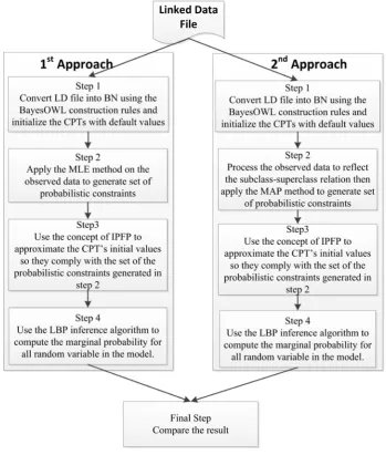
in such a way that it shows the effects of integrating the logical relations between random variables in BN. As a matter of fact, it compares the output of the Loopy Believe Propagation (LBP) inference algorithm using two different sets of probabilis-tic constraints. The first set ignores the logical relations between random variables while the second set accommodates these relations. Consequently, each data-set is processed in two different ways and the final results have been compared. Figure (3) shows the process sequence and the actions taken in each approach.

5.1 Preliminaries and Notations

Figure 3 shows that each data-set has been process in two differnt approaches. The first approach ignor the semantic relations between random variables while the second approach integrate these relations. Table (7) explains in details the steps on each approach.

Table 7. Proces walkthrough

Steps 1st approach 2nd approach

1 Convert the LD file into BN using the construction rules explained in section 2 and initialized the associated CPT’s with default value (i.e. 0.5).

2

Calculate the probabilistic con-straints using the MLE techniques base on the following equation.

𝑀𝑀𝐿𝐿𝐸𝐸= M1 /M1+M2 (6)

Where:

• M1 is the number of true trial.

• M2 is the number of false trial.

• Process the o observed data in such a way that reflect the superclass-subclass relations. In simple words, an instance of each class is observed as an instance of its superclass.

• Calculate the probabilistic constraints using the MAP techniques based on the following equation.

𝑀𝑀𝑀𝑀𝑀𝑀= (M1 +⍺−1) / (M1+⍺+M2+β−2) (7) Where:

• M1 is the number of true trial.

• M2 is the number of false trial.

• _⍺ is the number of true trail in the se-mantic data-set.

• β is the number of false trial in the semantic data-set.

3 Approximate the CPT’s initial values using the concept of IPFP and the set of constrains calculated in step 2.

4 Calculate the marginal probability for all random variable using the LBP infer-ence algorithm.

Table (7) clearly shows that steps 1, 3 and 4 are identical. However, the calculation of the probabilistic constraints in step 2 is differ . Hence, the input for steps 3 and 4 is changed accordingly. As a matter of fact, ⍺ and β hayperparameters in equation 7 were used to cater for the semantic relation other than the superclass-subclass rela-tions. These parameters utilized to inject the semantic relation into the estimation process.

5.2 Examples

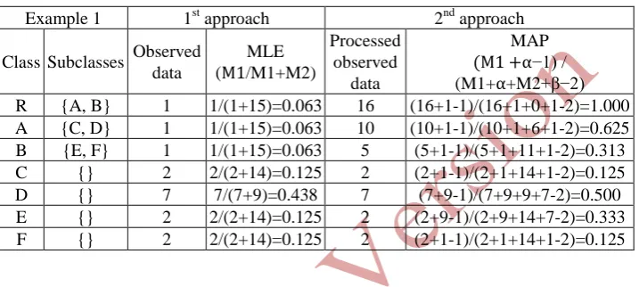
Example One (Equivalent of logical relation).

Figure 4.a indicates that class D is equivalent to class E. Hence, any instance of D is an instance of E and vice versa. Furthermore, it shows the superclass-subclass rela-tions between variables (i.e. classes) in example one. Table 8 illustrates the calcula-tion of the probabilistic constraints for the 1st and 2nd approach.

Table 8. Example one 1st approach Vs 2nd approach constraints calculations

Example 1 1st approach 2nd approach Class Subclasses Observed

data

MLE (M1/M1+M2)

Processed observed

data

MAP

(M1 +⍺−1) /

(M1+⍺+M2+β−2) R {A, B} 1 1/(1+15)=0.063 16 (16+1-1)/(16+1+0+1-2)=1.000 A {C, D} 1 1/(1+15)=0.063 10 (10+1-1)/(10+1+6+1-2)=0.625 B {E, F} 1 1/(1+15)=0.063 5 (5+1-1)/(5+1+11+1-2)=0.313 C {} 2 2/(2+14)=0.125 2 (2+1-1)/(2+1+14+1-2)=0.125 D {} 7 7/(7+9)=0.438 7 (7+9-1)/(7+9+9+7-2)=0.500 E {} 2 2/(2+14)=0.125 2 (2+9-1)/(2+9+14+7-2)=0.333 F {} 2 2/(2+14)=0.125 2 (2+1-1)/(2+1+14+1-2)=0.125

Discussions.

Table 8 shows how the observed data has been process to reflect the subclass-superclass relations. Additionally, it explains how the hayperparameters have been used to inject the semantic relations into the estimation process. For example, the value of ⍺ hayperparameter for class D and E is equal to 9, which is the sum of

the D and E instance because they are equivalent.

Figure 4.b clearly shows that the results of the second technique (i.e MAP) have re-flected the semantic relations between the random variables in example one. For ex-ample, the marginal probabilities for classes D and E, which were involved in the equivalent semantic relation, have increased compared to their marginal probabilities in the first approach. Likewise, the marginal probabilities for all classes involved in superclass-subclass relation were increased accordingly.

Example two (disjoint with logical relation).

Table 9. Example two 1st approach Vs 2nd approach constraints calculations

Example 2 1st approach 2nd approach Class

Sub-classes

Observed data

MLE (M1/M1+M2)

Processed observed

data

MAP

(M1 +⍺−1) / (M1+⍺+M2+β−2)

R {A, B} 1 1/(1+24)=0.040 25 (25+1-1)/(25+1+0+1-2)= 1.000 A {C, D} 3 3/(3+22)=0.120 9 (9+9-1)/(9+9+16+1-2) = 0.515 B {E} 5 5/(5+20)=0.200 15 (15+15-1)/(15+15+10+1-2)= 0.744 C {} 2 2/(2+23)=0.080 2 (2+2-1)/(2+2+23+8-2) = 0.091 D {} 4 4/(4+21)=0.160 4 (4+4-1)/(4+4+21+6-2) = 0.212 E {F,H} 6 6/(6+19)=0.240 10 (10+10-1)/(10+10+15+6-2)=0.487 F {} 2 2/(2+23)=0.080 2 (2+2-1)/(2+2+23+14-2)= 0.077 H {} 2 2/(2+23)=0.080 2 (2+2-1)/(2+2+23+14-2)= 0.077

Discussion.

Table 9 illustrates how the observed data has been processed to reflect the superclass-subclass relations. Furthermore, it shows how the value of β changes to accommodate the disjoint relations. For example, for class C the value of β is equal to 8, which means, the possibility that an instance belong to class C workspace but not an instance of class C it only could be an instance of class R, A or D because class A is disjoint with class B and its subclasses.

Figure 4.d compares between the marginal probabilities for all random variables in exampole two with and without considering the semantic relations between these variables. It can be seen that the marginal probability for classes A, B and their subclasses have accomodate the disjoint semantic relation.

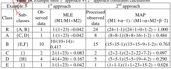
Example three (Complement of logical relation).

This example simulates the complement of semantic relation. Figure 4.e shows that class A is complement of class B. The semantic effect of this relation is that an in-stance of class A and its subclasses cannot be an inin-stance of class B and its sub-classes. Likewise, an instance of class B and its subclasses cannot be an instance of class A and its subclasses. Table 10 below explains the observed data processing step and the constraints estimation with and without injecting the semantic relation be-tween classes in example three.

Table 10. Example three 1st approach Vs 2nd approach constraints calculations

Example 3 1st approach 2nd approach Class

Sub-classes Ob-served

data

MLE (M1/M1+M2)

Processed observed

data

MAP

(M1 +⍺−1) / (M1+⍺+M2+β−2)

R {A, B} 1 1/(1+23) =0.042 24 (24+1-1)/(24+1+0+1-2) = 1.000 A {C, D} 1 1/(1+23) =0.042 8 (8+8-1)/(8+8+16+1-2) = 0.484

B {E,F} 10 10/(10+14)=

F {} 4 4/(4+20) = 0.167 4 (4+4-1)/(4+4+20+12-2) = 0.184 H {} 1 1/(1+23) = 0.042 1 (1+1-1)/(1+1+23+8-2) = 0.032

Discussion.

The hayperparameter β used to reflect the effect of the complement relation between class A and B. For example, the value of β for class H is equals to 8 which means an instance which is belong to H workspace and not an instance of class H, it only could be an instance of R, A, C or D because class A is complement of class B.

Figure 4.f shows the differences in marginal probabilities for all variables in example three when the semantic relations have been injected in the computation process and when they have been ignored. It shows that classes A, B and their subclasses have reflected the complement of semantic relation.

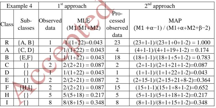
Example four (union of logical relation).

This example explains the union of logical relation. Figure 4.g shows that class E is the union of class H and I. The semantic interpretation of this relation is that any in-stance of H or I is an inin-stance of E as well. Table 11 explains the probabilistic con-strains calculation process with and without considering the union of the semantic relation between classes in example four.

Table 11. Example four 1st approach Vs 2nd approach constraints calculations

Example 4 1st approach 2nd approach Class

Sub-classes

Observed data

MLE (M1/M1+M2)

Pro-cessed observed

data

MAP

(M1 +⍺−1) / (M1+⍺+M2+β−2)

R {A, B} 1 1/(1+22)=0.043 23 (23+1-1)/(23+1+0+1-2) = 1.000 A {C, D} 1 1/(1+22) = 0.043 4 (4+1-1)/(4+1+19+1-2) = 0.174 B {E,F} 1 1/(1+22) = 0.043 18 (18+1-1)/(18+1+5+1-2) = 0.783 C {} 2 2/(2+21) = 0.087 2 (2+1-1)/(2+1+21+1-2)=0.087 D {} 1 1/(1+22) = 0.043 1 (1+1-1)/(1+1+22+1-2)=0.043 E {} 2 2/(2+21) = 0.087 2 (2+15-1)/(2+15+21+8-2)=0.364 F {H,I} 2 2/(2+21) = 0.087 15 (15+1-1)(15+1+8+1-2)=0.652 H {} 5 5/(5+18) = 0.217 5 (5+1-1)/(5+1+18+1-2)=0.217 I {} 8 8/(8+15) = 0.348 8 (8+1-1)/(8+1+15+1-2)=0.348

Discussion.

Table 11 shows how the ⍺ hayperparameter utilized to inject the union relation in

the estimation process. For example, the value of ⍺ for class E is equal to 15

which is the sum of the instances for classes H, I and E. This technique reflect the union relation which says that class E is the union of H and I. So, any instance of H and I is an instance of E as well.

the union relation has reflect the effect of this relation. Additionally, the effect of the superclass-subclass relations has been accommodated as well.

Example five (intersection of logical relation).

This example discusses the intersection of semantic relations. Figure 4.i shows that the class H is the intersection of class E and F. So, semantically this relation means that any instance of class H is an instance of class E and F. Table 12 compares be-tween calculating the probabilistic constraints with and without considering the se-mantic relations for random variable in example five.

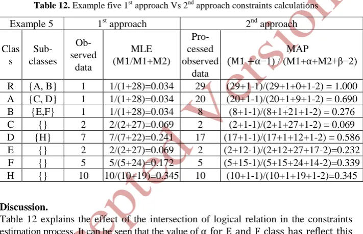
Table 12. Example five 1st approach Vs 2nd approach constraints calculations

Example 5 1st approach 2nd approach Clas

s

Sub-classes

Ob-served

data

MLE (M1/M1+M2)

Pro-cessed observed

data

MAP

(M1 +⍺−1) / (M1+⍺+M2+β−2)

R {A, B} 1 1/(1+28)=0.034 29 (29+1-1)/(29+1+0+1-2) = 1.000 A {C, D} 1 1/(1+28)=0.034 20 (20+1-1)/(20+1+9+1-2) = 0.690 B {E,F} 1 1/(1+28)=0.034 8 (8+1-1)/(8+1+21+1-2) = 0.276 C {} 2 2/(2+27)=0.069 2 (2+1-1)/(2+1+27+1-2) = 0.069 D {H} 7 7/(7+22)=0.241 17 (17+1-1)/(17+1+12+1-2) = 0.586 E {} 2 2/(2+27)=0.069 2 (2+12-1)/(2+12+27+17-2)=0.232 F {} 5 5/(5+24)=0.172 5 (5+15-1)/(5+15+24+14-2)=0.339 H {} 10 10/(10+19)=0.345 10 (10+1-1)/(10+1+19+1-2)=0.345

Discussion.

Table 12 explains the effect of the intersection of logical relation in the constraints estimation process. It can be seen that the value of ⍺ for E and F class has reflect this

relation. For example, the value of ⍺ for class E is equal to 12 which is the sum of

the instances for class H and E. Likewise; the value of ⍺ for class F is equal to 15.

6

Conclusions

The integration of data semantics in the mining process is not a new concept. Howev-er, exploiting the semantic relation in LD via the mining process is a new research area. LD not only intertwines the data and it’s semantic in one package, but also facil-itates the integration of various data-sets from multiple domains.

One major drawback of the conventional mining algorithms is transforming the LD original format into a format understandable by the mining algorithm. Accordingly, they cannot benefit from the semantical and structural features of the LD. To this end, this paper proposed a semantic-aware Bayesian network model which exploits the semantic nature of LD and implicitly accommodates the data intelligence in the min-ing process. Furthermore, it does not change the original format of the LD. So, linkmin-ing multiple data-sets is easily achievable.

The proposed approach consists of the following steps:

1. Convert the LD file into a BN which preserve the semantic of the original LD file. 2. Initialize the Conditional Probability Tables (CPT’s) with default value.

3. Calculate set of probabilistic constraints using the concept of Maximum a Posterior Estimation (MAP) in such a way that reflect the semantic relation between nodes in the BN.

4. Approximate the CPT’s initial values using the concept of Iterative Proportional Fitting Procedure (IPFP) and the set of probabilistic constraints estimated in the third step.

The proposed model has been tested using five sets of synthesized data. Each data-set highlight the significance of one logical relation. Initial results show that injecting the semantically aware probabilistic information into the Bayesian inference algorithm generates more realistic results.

Taking into account the fast accumulation of LD, this paper has investigated the suit-ability of Bayesian network for LD mining. Although synthesized data-set shows some promising results, the proposed model will be tested on real life data-set.

References

1. Fayyad, U., Piatetsky-Shapiro, G., Smyth, P.: From data mining to knowledge discov-ery in databases. AI Mag. 37–54 (1996).

2. Zhang, C., Zhang, S.: Association Rule Mining: Models and Algorithms. Springer-Verlag Berlin Heidelberg. XII, 244. (2002).

3. Cao, L., Yu, P.S., Zhang, C., Zhao, Y.: Domain driven data mining. Springer US.XVI, 248. (2010).

4. Cao, L.: Domain-driven data mining: Challenges and prospects. IEEE Trans. Knowl. Data Eng. 22, 755–769 (2010).

5. Sexton, M., Lu, S.: The challenges of creating actionable knowledge: an action re-search perspective. Constr. Manag. Econ. 2, 683–694 (2009).

dis-covering association rules in the skeletal dysplasia domain. J. Biomed. Semantics. 5, 8 (2014).

7. Dahan, H., Cohen, S., Rokach, L., Maimon, O.: Proactive Data Mining with Decision Trees. Springer New York (2014).

8. Antunes, C., Silva, A.: New Trends in Knowledge Driven Data Mining a position paper. Proc. 16th Int. Conf. Enterp. Inf. Syst. 346–351 (2014).

9. Bizer, C., Heath, T., Berners-Lee, T.: Linked data-the story so far. Int. J. Semant. Web Inf. Syst. 5, 1–22 (2009).

10. Quboa, Q.K., Saraee, M.: A State-of-the-Art Survey on Semantic Web Mining. Intell. Inf. Manag. 05, 10–17 (2013).

11. Ding, Z., Peng, Y., Pan, R.: BayesOWL : Uncertainty Modelling in Semantic Web

Ontologies. Soft Comput. Ontol. Semant. Web. 204, 3–29 (2006).

12. Ma, Z.: Soft Computing in Ontologies and Semantic Web. Springer Sci. Bus. Media. (2007).

13. Sun, Y.: A Prototype Implementation of BayesOWL ,Diss. University of Mayryland Baltimore County, (2009).

14. Ding, Z.: BayesOWL, http://www.csee.umbc.edu/~ypeng/BayesOWL/index.html.

15. Ding, Z., Peng, Y.: A Bayesian approach to uncertainty modelling in OWL ontology, MARYLAND UNIV BALTIMORE DEPT OF COMPUTER SCIENCE AND ELECTRICAL ENGINEERING.,(2006).

16. Zhang, S., Sun, Y., Peng, Y., Wang, X.: A Practical Tool for Uncertainty in OWL Ontologies. Proc. 10th IASTED Int. Conf. 674, 235.

17. Koller, D., Friedman, N.: Probabilistic Graphical Models Principles and Techniques. MIT press (2009).

18. Jensen, F. V., Nielsen, T.D.: Bayesian Networks and Decision Graphs. Springer Sci-ence & Business Media (2009).

19. Almond, R.G., Mislevy, R.J., Steinberg, L.S., Yan, D., Williamson, D.M.: Learning in Models with Fixed Structure. Bayesian Networks Educ. Assessment. Springer New York. 279–330 (2015).

20. Heinrich, G.: Parameter estimation for text analysis. Tech. Report, Fraunhofer IGD, Darmstadt, Ger. (2005).

21. Levy, R.: Probabilistic Models in the Study of Language , Diss,University of Califor-nia, San Diego, (2012).

22. Fienberg, S.E.: An iterative procedure for estimation in contingency tables. Ann. Math. Statisitics. 907–917 (1970).

23. Cramer, E.: Probability measures with given marginals and conditionals: I-projections and conditional iterative proportional fitting. Stat. Decis. J. Stoch. Methods Model. 311 – 330 (2000).