A Comparative Study of Active-Learning Techniques for Classification of Remote Sensing Images

International Journal of Emerging Technology and Advanced Engineering

A Comparative Study of Active-Learning Techniques for

Classification of Remote Sensing Images

Janardhana Bhat K1, Venugopala P.S2 1

Faculty, Dept. of Computer Science & Engg., Srinivas Institute of Technology,Mangalore, Karnataka

2

Assistant Professor, Dept. of Computer Science & Engg., NMAMIT, Nitte, Karkala, Karnataka Abstract— The success of remote sensing image

classification techniques is based on defining an efficient training set. Active learning aims at building efficient training sets by iteratively improving the model performance through sampling.

Active learning is an active research area within the machine learning community, and is now being extensively used for remote sensing applications. To make remote sensing image classification effective the training set should be as small as possible and must include highly informative pixels. Active learning heuristics provide capability to select “most informative” unlabeled data and to obtain the respective labels, fulfilling both goals. The investigated techniques exploit different query functions, which are based on the evaluation of two criteria: uncertainty and diversity. The combination of the two criteria results in the selection of the potentially most informative set of samples at each iteration of the AL process. This paper investigates different active learning (AL) techniques for the classification of remote sensing (RS) images with support vector machines.

Index Terms—Active Learning, Classification, Support

Vector Machines (SVM), Margin Sampling (MS), Entropy Query by Bagging (EQB), Multiclass Level Uncertainty (MCLU), Angle Based Diversity (ABD)

I. INTRODUCTION

For the classification of Remote Sensing Images several supervised methods have been proposed in different Remote sensing literature. In all these methods to train the classifier labeled samples are necessary, and the classification results rely on the quality of the labeled samples used for learning. However, the collection of labeled samples is time consuming and costly, and the available training samples are often not enough for an adequate learning of the classifier. Moreover, inclusion of redundant samples in the training set slows down the training step of the classifier without adding information. In order to reduce the cost of labeling, the training set should be kept as small as possible, avoiding redundant samples and including patterns which contain the largest amount of information and thus can optimize the performance of the model.

Semisupervised learning and active learning are the two popular machine learning approaches for dealing with drawbacks of supervised methods. Semisupervised algorithms incorporate the unlabeled data into the

classifier training phase to obtain more precise decision boundaries.

In active learning, the learning process repeatedly queries unlabeled samples to select the most informative samples and updates the training set on the basis of a supervisor who attributes the labels to the selected unlabeled samples. In this way, unnecessary and redundant samples are not included in the training set, thus greatly reducing both the labeling and computational costs. This is particularly important for remote sensing images that may have highly redundant pixels.

II. ACTIVE LEARNING

Defining an efficient training set is one of the most delicate phases for the success of remote sensing image classification routines. The goal of Active learning [1], is to build efficient training sets by iteratively improving the model performance through sampling. A user-defined heuristic ranks the unlabeled pixels according to a function of the uncertainty of their class membership and then the user is asked to provide labels for the most uncertain pixels.

A general active learner can be modeled as a quintuple (G, Q, S, L, and U). G is a classifier, which is trained on the labeled samples in the training set L. Q is a query function used to select the most informative samples from an unlabeled sample pool U. S is a supervisor who can assign the true class label to the selected samples from U. Initially, the training set L has few labeled samples to train the classifier G. After that, the query function Q is used to select a set of samples from the unlabeled pool U, and the supervisor S assigns a class label to each of them. Then, these new labeled samples are included into L, and the classifier G is retrained using the updated training set. The closed loop of querying and retraining continues for some predefined iterations or until a stop criterion is satisfied.

Algorithm 1 gives a description of a general active-learning process.

Algorithm 1: Active-learning process

Step 1: Train the classifier G with the training set L

International Journal of Emerging Technology and Advanced Engineering

336 Repeat

Step 2: Select a set of samples from the unlabeled pool U using the query function Q.

Step 3: Assign class label to each of the acquired samples by a supervisor S.

Step 4: Add the new labeled samples to the training set L.

Step 5: Retrain the classifier G. Until the stop criterion is satisfied.

The query function is fundamental in the active-learning process. In [3], several methods have been proposed in the machine learning literatures which differ only in their query functions, and these different query functions are based on the evaluation of two criteria: uncertainty and diversity. The uncertainty criterion is associated to the confidence of the supervised algorithm in correctly classifying the considered sample, while the diversity criterion aims at selecting a set of unlabeled samples that are as more diverse (distant one another) as possible, thus reducing the redundancy among the selected samples. The combination of the two criteria results in the selection of the potentially most informative set of samples at each iteration of the AL process.

III. METHODOLOGIES

Different strategies have been proposed in the literature for the active selection of training examples. The following sections present the MS algorithm and the active learning approaches proposed in this paper.

A. Support Vector Machine (SVM)

The basic SVM takes a set of input data and predicts, for each given input, which of two possible classes forms the output. Assumption is that a training set consists of N labeled samples (xj, yj) for j=1 to N, where

xj Є Rd denotes the training samples and yj Є {+1,−1} denotes the associated labels (which model classes ω1 and ω2). The goal of a binary SVM is to find out a hyperplane that separates the d-dimensional feature space into two subspaces (one for each class).

An interesting feature of SVMs is related to the possibility to project the original data into a higher dimensional feature space via a kernel function K(., .).

The decision function f(x) is defined as,

f(x) =∑xj є SVαjyj K(xj, qi) + b (1)

where SV represents the set of support vectors. The training pattern xj is a support vector if the corresponding

αj has a nonzero value. For a given test sample qi, the sign of the discriminant function f(qi) defined in [4] is used to predict its class label.

B. Margin Sampling (MS)

MS is a SVM-specific active learning algorithm taking advantage of SVM properties.

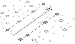
Assuming a linearly separable case, where the two classes are separated by a hyperplane given by the SVM classifier [Fig.1], the support vectors are the labeled examples that lie on the margin at a distance of exactly 1 from the decision boundary (filled circles and diamonds in Fig.1). If we now consider an ensemble of unlabeled candidates (“X”s in Fig.1), we make the assumption that the most interesting candidates are the ones that fall within the margin of the current classifier, as they are the most likely to become new support vectors [Fig.1].

Fig.1. MS active learning, (Left) SVM before inclusion of the two most interesting examples, (Right) New SVM decision boundary

after inclusion of the new training examples.

As mentioned earlier the sign of discriminant function (1) f(qi) is used to predict its class label. In a multiclass context and using a one-against-all SVM [2], a separate classifier is trained for each class cl against all the others, giving a class-specific decision function fcl(qi). The class attributed to the candidate x is the one minimizing fcl(qi).

Therefore, the candidate included in the training set is the one that respects the condition

x = arg min |f(qi)| (2) qi є Q

In the case of remote sensing imagery classified with SVM, the inclusion of a single candidate per iteration is not optimal. Considering computational cost of the model (cubic with respect to the observations), inclusion of several candidates per iteration is preferable. MS provides a set of candidates at every iteration. However, MS has not been designed for this purpose, and such a straightforward adaptation of the method is not optimal on its own. The Fig. 2 shows the effect of a nonuniform distribution of candidates when several neighboring examples lie close to the margin: if the MS algorithm chooses three examples in a single run, three candidates from the same neighborhood will be chosen.

International Journal of Emerging Technology and Advanced Engineering

Fig. 2. MS active learning, Candidates chosen by the MS.

C. Entropy-query-by-bagging (EQB)

The query-by-bagging approach is quite different from the approaches discussed previously. In query-by-committee algorithms, the choice of a candidate is based on the maximum disagreement between a committee of classifiers. In the implementation of the approach in [6], bagging is proposed to build the committee: first, k

training sets built on bootstrap samples, i.e., a draw with replacement of the original data, are defined. Then, each set is used to train a SVM classifier and to predict the class membership of the m candidates. At the end of the bagging procedure, k possible labelings of each candidate are provided. The approach proposed in [6] has been discussed for binary classification: the candidates that will be added to the training set are the ones for which the predictions are the most evenly split, as shown in

x= arg min|| {t ≤ k|ft(qi) = 1} |−|{t ≤ k|ft(qi) = 0} || (3) qiєQ

where t is one of the k classifiers and the binary labels are of the form {0, 1}. If the classifiers agree to a certain classification, (3) is maximized. On the contrary, uncertain candidates yield small values.

In paper [5], the heuristic of (3) is replaced by a multiclass one based on the maximum entropy of the distribution of the predictions of the k classifiers [see (5)]. By considering the k labels of a given candidate qi, it is possible to compute the entropy of the distribution of the labels H(qi) using

where pi, cl is the probability to have the class cl

predicted for the candidate i. H(qi) is computed for each candidate in Q, and then, the candidates satisfying the heuristic

are added to the training set.

Entropy maximization gives a naturally multiclass heuristic. A candidate for which all the classifiers in the committee agree is associated with null entropy; such a candidate is already correctly labeled by the classifiers,

and its inclusion does not bring additional information. On the contrary, a candidate with maximum disagreement between the classifiers results in maximum entropy, i.e., a situation where the predictions given by the k classifiers are the most evenly split. Therefore, the parallels with the original query-by-bagging formulation are strong.

The EQB does not depend on SVM characteristics but on the distribution of k class memberships resulting from the committee learning. Therefore, it depends on the outputs of the classifiers only and can be applied to any type of classifier.

Regarding computational cost of the method, some specific considerations can be done depending on the classifier used: when using a SVM, the cost remains competitive compared to the MS presented earlier, because the training phase scales linearly with respect to the number of models k (when all the training sets are drawn in the bootstrap samples) compared to the MS using the entire training set.

D. Multiclass Level Uncertainty (MCLU)

The adopted Multiclass Level Uncertainty (MCLU) technique selects the most uncertain samples according to a confidence value c(x), x є U, which is defined on the basis of their functional distance fi(x), i = 1, . . . , n, to the n decision boundaries of the binary SVM classifiers included in the OAA architecture [5], [7]. In this technique, the distance of each sample x є U to each hyperplane is calculated, and a set of n distance values

{f1(x), f2(x), . . . , fn(x)} is obtained. Then, the confidence value c(x) can be calculated using different strategies. The strategy used in the current work is, the difference function cdiff strategy, which considers the difference between the first and second largest distance values to the hyperplanes [7], i.e.,

The function models a simple strategy that computes the confidence of a sample x, taking into account the minimum distance to the hyperplanes evaluated on the basis of the most uncertain binary SVM classifier. Differently, the cdiff(x)strategy assesses the uncertainty between the two most likely classes. If this value is high, the sample x is assigned to r1maxwith high confidence. On the contrary, if cdiff(x)is small, the decision for r1max is not reliable, and there is a possible conflict with the class r2max. Thus, this sample is considered uncertain and is selected by the query function for better modeling the decision function in the corresponding position of the

x = arg max H(qi) (5) qiєQ

H(qi)=∑cl –pi,cl log(pi,cl) (4)

= arg max

. …., { ( )}

= arg max

. …., ,

( ) = ( )− ( ) ₍₆₎

International Journal of Emerging Technology and Advanced Engineering

338 feature space. These c(x) value of each x є U is obtained based on one of the two aforementioned strategies, the m

samples x1MCLU,x2MCLU,…..,xmMCLU denote the selected most uncertain samples based on the MCLU strategy [3].

E. MS-Angle Based Diversity (ABD)

In [8], the first heuristic was proposed where the diversity criteria in remote sensing is found. The measure of angle between candidates in feature space constraints the margin sampling heuristic. The heuristic starts from the samples selected by MS, UMS ⊂ U, the diversity criteria iteratively chooses the samples minimizing the highest values between the candidates list and the samples already included in the batch S. This iterative heuristic is called “most ambiguous and orthogonal” (MAO). For a single iteration, this can be given as [1],

F. MCLU-ABD

In the binary AL algorithm, the uncertainty and ABD criteria are combined based on a weighting parameter λ

as presented in [9]. On the basis of this combination, a new sample xt is included in the selected batch X

according to the following optimization problem [3]:

where I denotes the set of unlabeled examples whose distance to the classification hyperplane is less than one, i.e., I = {xi є U : |f(xi)| <1}, I/X represents the set of unlabeled samples of I that are not contained in the current batch X, and λ provides the trade off between uncertainty and diversity. The cosine angle distance between each sample in I/X and the samples included in

X is calculated, and the maximum value is taken as the diversity value of the corresponding sample. Then, the sum of the uncertainty and diversity values weighted by

λ is considered to define the combined value. The unlabeled sample xt that minimizes such value is

included in X. This process is repeated until the number of samples of the set X (|X|) is equal to h. This technique guarantees that the selected unlabeled samples in X are diverse regarding their angles to all the others in the kernel space. Since the initial size of X is zero, the first sample included in X is always the most uncertain sample of I (i.e., the sample closest to the hyperplane).

IV. DATA SETS AND SETUP

A.Indian Pines

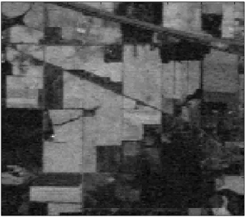
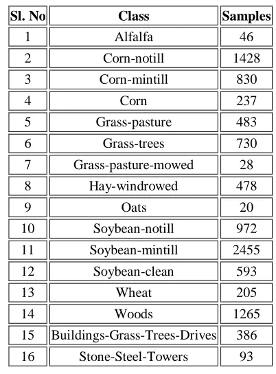
The Indian Pines scene, shown in Fig. 3(a), was gathered by AVIRIS sensor over the Indian Pines test site in North-western Indiana and consists of 145\times145 pixels and 224 spectral reflectance bands in the wavelength range 0.4–2.5 10^(-6) meters. This scene is a subset of a larger one. The Indian Pines scene contains two-thirds agriculture, and one-third forest or other natural perennial vegetation. There are two major dual lane highways, a rail line, as well as some low density housing, other built structures, and smaller roads. Since the scene is taken in June some of the crops present, corn, soybeans, are in early stages of growth with less than 5% coverage. The groundtruth, shown in Fig. 3(b), available is designated into sixteen classes, given in TABLE I, and is not all mutually exclusive. We have also reduced the number of bands to 200 by removing bands covering the region of water absorption: [104-108], [150-163] 220.

Fig. 3(a). Sample band of Indian Pines Dataset

Fig. 3(b). Groundtruth of Indian Pines Dataset

= arg min

∈ max∈ ,

^ (7)

= arg min ∈ ⁄ | ( )| +(1− ) × max ∈

International Journal of Emerging Technology and Advanced Engineering

TABLE I.

Groundtruth Classes For The Indian Pines Scene And Their Respective Samples Number.

Sl. No Class Samples

1 Alfalfa 46

2 Corn-notill 1428

3 Corn-mintill 830

4 Corn 237

5 Grass-pasture 483

6 Grass-trees 730

7 Grass-pasture-mowed 28

8 Hay-windrowed 478

9 Oats 20

10 Soybean-notill 972

11 Soybean-mintill 2455

12 Soybean-clean 593

13 Wheat 205

14 Woods 1265

15 Buildings-Grass-Trees-Drives 386

16 Stone-Steel-Towers 93

B.Salinas Scene

The Salinas scene was also collected by the 224-band AVIRIS sensor over Salinas Valley, California, and is characterized by high spatial resolution (3.7-meter pixels). The area covered comprises 512 lines by 217 samples. As with Indian Pines scene, the 20 water absorption bands have been discarded, in this case bands: [108-112], [154-167], 224. This image was available only as at-sensor radiance data. It includes vegetables, bare soils, and vineyard fields. Salinas’s groundtruth contains 16 classes.

In this paper, a small subscene of Salinas image, shown in Fig. 4(a), denoted Salinas-A, is used. It comprises 86*83 pixels located within the same scene at [samples, lines] = [591-676, 158-240] and groundtruth, shown in Fig. 4(b), of Salinas-A includes six classes (given in TABLE II).

C.Experimental Setup

In the experiments, SVM classifiers with RBF kernel classifiers have been considered for the experiments. When using SVM, free parameters have been optimized by ten-fold cross validation optimizing an accuracy criterion. The active learning algorithms have been run in two settings, adding N+5 and N+10 pixels per iteration. To reach convergence, 80 (40 in the case N+10) iterations have been executed for both the images.

The classification accuracy has been computed by considering a model trained on the whole set (“Standard SVM”). The results of these models have been compared against the result obtained by considering a model using an increasing training set, randomly adding the same number of pixels at each epoch (“Random Sampling”).

Fig. 4(a). Sample band of Salinas-A Dataset

Fig. 4(b). Groundtruth of Salinas-A Dataset

TABLE II.

Groundtruth Classes For The Salinas-A Scene And Their Respective Samples Number

Sl.No Class Samples

1 Brocoli_green_weeds_1 391

2 Corn_senesced_green_weeds 1343

3 Lettuce_romaine_4wk 616

4 Lettuce_romaine_5wk 1525

5 Lettuce_romaine_6wk 674

International Journal of Emerging Technology and Advanced Engineering

340 V. RESULTS

In this section the different heuristics discussed are studied on the two datasets presented above. Here an effort is made to illustrate the potential of the different methods. The base learner used in the experiment is SVM classifier and the heuristics studied are: MS, MCLU, MS-ABD, MCLU-ABD and EQB. The results are compared with Random Sampling (RS).The experiments were run with 10 fold cross validation.

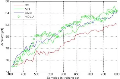
In Fig. 5 the result of uncertainty heuristics examined on Indian Pines dataset are compared using SVM classifiers. On Indian Pines dataset the overall performance of MCLU is better compared to other uncertainty criterions considered. The confidence value is calculated with the cdiff(x) strategy for MCLU, because the effectiveness of cdiff(x) uncertainty method is superior compared to cmin(x) strategy. The performance of MS is also close to the performance of MCLU. The reason is, in MS the candidates are ranked directly using the SVM classifier function with no further estimations. Slightly reduced performance of the EQB is due to the small size of the initial training set. In both of the experimental set up, N+5 and N+10 (shown in Fig. 5(a) and Fig. 5(b)) the performances of uncertainty methods are very similar.

In Fig. 6 with Salinas-A dataset the overall performance of MCLU is still better compared to other uncertainty criterions considered. RS is performing reasonably well, but MS does not perform well at the beginning of the learning stage. But the performance of the MS and that of EQB are closer to each other.

(a) N+5 pixels per iteration

(b) N+10 pixels per iteration

Fig. 5: Result of uncertainty heuristics examined on Indian Pines dataset

(a) N+5 pixels per iteration

(b) N+10 pixels per iteration

International Journal of Emerging Technology and Advanced Engineering

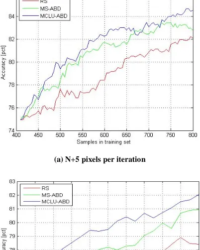
diversity criteria are illustrated. In Fig. 7 the result of uncertainty and diversity heuristics are examined on Indian Pines dataset. It can be observed that the effectiveness of the MCLU-ABD is better compared to MS and MCLU without considering the diversity criterion. The performance of MS-ABD is also close enough to the performance of MCLU-ABD. There exists some added computational cost involved in the improvement of the performance when diversity criterion is used.

In Fig. 8the result of uncertainty and diversity heuristics are examined on Salinas-A dataset. In the result obtained again MCLU-ABD is performing well. But MS-ABD does not perform well at the beginning of the learning stage. But as the number of training samples increases, one can observe the gradual rise in accuracy of MS-ABD, which is expected to converge with RS.

(a) N+5 pixels per iteration

(b) N+10 pixels per iteration

Fig. 7: Result of uncertainty and diversity heuristics examined on Indian Pines dataset.

(a) N+5 pixels per iteration

(b) N+10 pixels per iteration

Fig. 8: Result of uncertainty and diversity heuristics examined on Salinas-A dataset.

VI. CONCLUSION

International Journal of Emerging Technology and Advanced Engineering

342 REFERENCES

[1] D. Tuia, M. Volpi, L. Copa, M. Kanevski, and J. Mu˜noz-Mar´ı,

“A survey of active learning algorithms for supervised remote sensing image classification,” IEEE J. Sel. Topics Signal Proc., vol. 5, no. 3, pp. 606–617, 2011.

[2] M. Li and I. K. Sethi, “Confidence-based active learning,” IEEE Trans. Pattern Anal. Mach. Intell., vol. 28, no. 8, pp. 1251–1261, Aug. 2006.

[3] B. Demir, C. Persello, and L. Bruzzone, “Batch mode active learning methods for the interactive classification of remote sensing images,” IEEE Trans. Geosci. Remote Sens., vol. 49, no. 3, pp. 1014–1032, 2011.

[4] S. Patra and L. Bruzzone, “A fast cluster-assumption based active-learning technique for classification of remote sensing images,” IEEE Trans. Geosci. Remote Sens., vol. 49, no. 5, pp. 1617–1626, 2011.

[5] D. Tuia, F. Ratle, F. Pacifici, M. F. Kanevski, and W. J. Emery, “Active learning methods for remote sensing image classification,” IEEE Trans. Geosci. Remote Sens., vol. 47, no. 7, pp. 2218–2232, Jul. 2009.

[6] N. Abe and H. Mamitsuka, “Query learning strategies using boosting and bagging,” in Proc. ICML, Madison, WI, 1998, pp. 1–9.

[7] A. Vlachos, “A stopping criterion for active learning,” Comput. Speech Lang., vol. 22, no. 3, pp. 295–312, Jul. 2008.

[8] M. Ferecatu and N. Boujemaa, “Interactive remote sensing image retrieval using active relevance feedback,” IEEE Trans. Geosci. Remote Sens., vol. 45, no. 4, pp. 818–826, Apr. 2007.