Image Segmentation for Text Recognition using Boundary Analysis.

(1)

International Journal of Emerging Technology and Advanced Engineering

Website: www.ijetae.com (ISSN 2250-2459,ISO 9001:2008 Certified Journal, Volume 4, Issue 2, February 2014)

294

Image Segmentation for Text Recognition using Boundary

Analysis.

Rohit Kolar

1

, Akshay Thakar

2

, Muzaffar Shabad

3 1,2

final year student of Universal College of Engineering & Research, Pune. 3_{lecturer at Universal College of Engineering & Research, Pune}

Abstract— This paper provides the theoretical bases for image segmentation based on boundary analysis and its application for text recognition. The first part of the article contains introduction of the image segmentation boundary analysis. We tried to elaborate the principal moments which allow to understand quickly enough an essence of the boundary analysis, and to begin its application in practice. In the rest of the part it contains some aspects of the theory, and optimization of algorithms of the boundary analysis.

Keywords— Complex numbers, Gray scale Image, Image binarization, Image segmentation, Scalar product.

I. INTRODUCTION

The system underlying the title concerns with Image segmentation. Image segmentation is the process of dividing a digital image into multiple parts i.e. segments. The purpose of segmentation is to make easy representation of an image which will in turn be meaningful and easier to analyze. It is generally used to make separation of individual objects in the Image. For the purpose of segmentation we need to analyze the pixel properties. More precisely, mage segmentation is the process of assigning a label to every pixel in an image such that pixels with the same label share certain visual characteristics.

After the segmentation is applied to the image we can see the result contains set of segments that collectively form the entire image, or a set of contours extracted from the image. Each pixel in a single segment share same characteristics such as color, intensity, or texture.

Adjacent regions are significantly different with respect to the same characteristics. Image segmentation can be done in two ways – (1) region-based, and (2) contour-based. Region-based approaches try to find partitions of the image pixels into sets corresponding to coherent image properties such as brightness, color and texture. Contour-based approaches usually start with a first stage of edge detection, followed by a linking process that seeks to exploit curvilinear continuity. In the proposed system we are going to concern with contour based approach i.e. Boundary Analysis.

II. BOUNDARY ANALYSIS BASICS

(2)

International Journal of Emerging Technology and Advanced Engineering

295

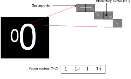
Figure (1) - Complex number encoding.

The boundarys of 3-dimentional objects are always closed and cannot have self-intersection. It allows to define unambiguously a way of bypass of a boundary (to within a direction - on or counter-clockwise). The last vector of a boundary always leads to the starting point. Each vector of a boundary we will name Elementary Vector (EV). And

sequence of complex-valued numbers – Vector

boundary (VC). Vector-boundarys we will designate the big Greek letters, and their elementary a vector - small Greek letters.

Thus, vector-boundary Γ of length k can be designated as:

Γ = (γ0, γ1, ….. γk-1)

In correlational algorithm complex number encoding is used, because operations over a boundary as over a vector of complex numbers possess remarkable mathematical properties, in comparison with other modes of coding. Basically, complex coding is close to two-dimensional coding where the boundary is defined as a population of the EVs presented in the two-dimensional coordinates.

But a difference between operation of scalar product for vectors and for complex numbers - are various. This circumstance also gives priority to CA methods.

III. PROPERTIES OF A BOUNDARY

A.The sum of an EV of a closed boundary is equal to zero. It is trivial - as the elementary vectors result in starting point, their sum is equal to a zero-vector. B.The boundary-vector does not depend on parallel

transposition of the source image. As the boundary is encoded relative to starting point, this mode of coding is invariant to shift of an initial boundary.

C.Image turn on certain angle is equivalent to turn off each EV of a boundary on the same angle.

D.The starting point modification conducts to VC cycle shift. As EVs are encoded concerning the previous point, it is clear that at a modification of starting point, the sequence of an EV will be the same, but the first EV will be what begins in the starting point. E.The source image rescaling can be considered as

[image:2.612.92.517.158.414.2]

(3)

International Journal of Emerging Technology and Advanced Engineering

296

IV. SCALAR PRODUCT OF BOUNDARY

As scalar product of boundarys, Γ and N are called such complex number:

η = (Γ, N) = (1)

Where k - dimensionality of a VC, γn - n the elementary vector of boundary Γ, νn - n EV of boundary N. (γn, νn) – the scalar product of complex numbers calculated as:

(a + ib, c+id) = (a + ib)(c + id) = ac + bd + i(bc – ad) (2)

Let's pay attention to that in a CA the scalar product only a VC of identical dimensionality is supposed. That is the number of the elementary vectors in boundarys should coincide. The scalar product of usual vectors and scalar product of complex numbers - differ. If we multiplied an EV as simple a vector, their scalar product would look so:

((a, b), (c, d)) = ac + bd

(3)

Compare this formula to the formula (2) and you note that:

A. Outcome of scalar product of vectors is the real number. And outcome of product of complex numbers - a complex number.

B. The real part of scalar product of complex numbers coincides with scalar product of appropriate vectors. That is complex product includes vectorial scalar product.

Now we consider linear algebra, to be exact - physical sense and properties of scalar product. The scalar product is equal in the linear algebra to product of lengths of vectors on a cosine of the angle in between. It means that two perpendicular vectors will always have zero scalar product, collinear a vector - opposite, will give maximum value of scalar product. These properties of product allow to use it as a certain measure of closeness of vectors. If it is more - the fewer angles between vectors, the "more close" they are to each other.

For perpendicular vectors - it is lowered to zero, and further becomes negative for the vectors directed every which way. It appears, scalar product (1) also possesses similar properties.

V. NORMALIZEDSCALAR PRODUCT (NSP)

η = (4)

Where |Γ| and |N| - the norms (length) of boundarys calculated as:

(5)

The NSP in space of complex numbers, also is a complex number. Thus, unity is greatest possible value of norm of NSP (it follows from a Cauchy–Bunyakovsky– Schwarz inequality: |ab| <= |a||b|), and it is reached only if...

= μN (6)

...Where μ - the arbitrary complex number.

(4)

International Journal of Emerging Technology and Advanced Engineering

297

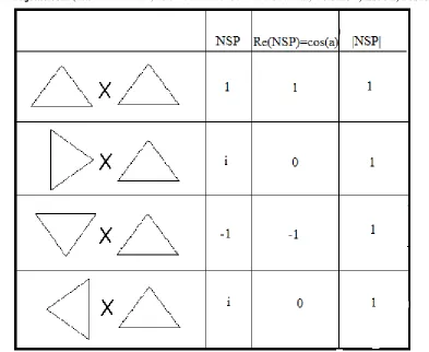
Figure (2) - Properties of the normalized scalar product of contours.

Similarly, if we scale the vector contour i.e. increase it by some real coefficient we also receive NSP=1. Transposition, rotation and scaling of boundarys are invariant to Norm of NSP. Even after the turn and scale norm of the NSP gives unity as a result. If the norm gives strict less unity then Vector contours are not identical. If there are two identical boundarys their NSP always gives a unity, is not dependent on where boundarys are, what their angle of rotation and a scale. Similarly, if boundarys are various, their NSP will be strict less 1, and also independent of a place, rotation and a scale. Norm of NSP is measure of boundarys closeness. The norm gives a measure of a likeness of boundarys, and argument a NSP (equal atan(b/a)) - gives us an angle of rotation of boundarys rather each other.

VI. CORRELATION FUNCTION OF BOUNDARY

In the previous section, we observed that the NSP is extremely useful formula for search of boundarys similar

among themselves. Unfortunately, there is one

circumstance not allowing to use it directly.

And this circumstance - a starting point choice. The matter is that the equality (6) is reached only if starting points of boundarys - coincide. If boundarys are identical, but the EV reference begins with other starting point the norm the NSP of such boundarys will not be equal to a unity.

The matter is that the equality (6) is reached only if starting points of boundarys - coincide. If boundarys are identical, but the EV reference begins with other starting point the norm the NSP of such boundarys will not be equal to a unity.

Let's introduce the concept of intercorrelation

function (ICF) of two boundarys:

τ (m) = (Γ,N(m)_{), m = 0, … , k-1 (7)}

Where N(m) - a boundary received from N by cycle shift by its EV on m of elements.

[image:4.612.111.504.128.450.2]

(5)

International Journal of Emerging Technology and Advanced Engineering

298

What does intercorrelation function show? Values of this function show boundarys Γ and N are how much similar if to shift starting point N on m positions. ICF it is defined on all set of integral numbers but as cycle shift on k leads us to an initial boundary the ICF is periodic, with phase k. Therefore us will interest values of this function only in limits from 0 to k-1.

Let's discover the magnitude having the maximum norm among values an ICF:

τmax = max , m = 0, …. , k-1 (8)

From determinations a NSP and an ICF, it is clear that τmax is a measure of similarity of two boundarys, invariant to transposition, scaling, rotation and starting point shift. Thus, the norm |τmax| shows a level of similarity of boundarys, and reaches unity for identical boundarys, and the argument arg(τmax) gives an angle of rotation of one boundary, concerning another. Maximum of norm of ICF is a measure of similarity of two boundarys.

Let's introduce one more concept - an autocorrelation function (ACF). The Autocorrelation function is an ICF for which N=Γ. As a matter of fact is a scalar product of a boundary most on itself at various shifts of starting point:

v(m) = (Γ, Γ(m) _{), m = 0, ….. , k-1 (9)}

Let's consider some properties an ACF:

A.The ACF does not depend on a choice of starting point of a boundary. Really, we look at determination of a scalar product (1). As we see, the starting point modification leads simply to a modification of the order of summable elements and does not result to a sum modification. This conclusion is not so obvious but if to ponder upon sense an ACF it is clear.

B.The norm an ACF is symmetric concerning a central reference k/2. As the ACF is the total of pairwise products of an EV of a boundary each pair meets two times on an interval from 0 to k.

Let, for example, N = (n1, n2, n3, n4), we write values an ACF for different m:

ACF(0)=(n1,n1)+(n2,n2)+(n3,n3)+(n4,n4)

ACF(1)=(n1,n2)+(n2,n3)+(n3,n4)+(n4,n1)

ACF(2)=(n1,n3)+(n2,n4)+(n3,n1)+(n4,n2)

ACF(3)=(n1,n4)+(n2,n1)+(n3,n2)+(n4,n3) ACF(4)=(n1,n1)+(n2,n2)+(n3,n3)+(n4,n4).

Let's note that items in an ACF (1) same, as in an ACF (3), to within permutation of factors. And recalling that for complex numbers (a, b) = (b, a)*, we receive that an ACF (1) = ACF (3)*, where * - a conjugate complex number sign. And as |a*| = |a| turns out that norms of ACF (1) and an ACF (3) - coincide.

Similarly, norms an ACF (0) and an ACF (4) coincide. Further, everywhere under an ACF we will understand only a function part on an interval from 0 to k/2 as the remaining part of function - is symmetric to the first part.

VII. CONCLUSION

In this paper we have elaborated the image segmentation using boundary analysis. We have included some unique properties of boundary which helps to extract it from the background in the image. Also we have put correlational algorithms such as ICF and ACF for comparison of two boundaries. This will in turn help us to recognize a text as a collection of individual alphabets and digits from the image. We hope that this paper will simplify the understanding of boundary analysis for image segmentation.

REFERENCES

[1] Linda G. Shapiro and George C. Stockman (2001): ―Computer Vision‖, pp. 279-325, ISBN.

[2] ―Current Methods in Medical Image Segmentation‖. Annual Review of Biomedical Engineering 2:315-337.Pham, Dzurng L.

[3] K J. Batenburg, and J. Sijibers, ―Adaptive threshholding of tomograms by projection distance minimization.