Incremental Feature Subsetting useful for Big Feature
Space Problems
P. Nagabhushan
Professor,
Dept of Studies in Computer Science, University of Mysore,
Karnataka, India
Preeti Mahadev
Research Scholar, Dept of Studies in Computer
Science, University of Mysore,
Karnataka, India
ABSTRACT
Dimensionality Reduction process is a means to overcome curse of dimensionality in general. When all features are available together, it is a way to extract knowledge from a population in a big feature space. On the contrary, dimensionality reduction is intriguing when update to feature space is streaming and the question arises whether one could reduce the feature space as and when the features become available instead of waiting for all the features to arrive .This could not only enable the creation of knowledge that can incrementally align with the incremental access to feature space, but would also facilitate decision making locally at every incremental stage. While facilitating the local decision making parameters, it would eventually generate the most optimal reduced feature space. Moving in this direction, the possibility of implementing feature subsetting in an incremental framework is explored. The incremental streaming could be due to the temporal arrival of features or due to collection of features arriving from distributed sources. In this paper, the adoption of incremental dimensionality reduction model is also explored to observe the complexity reduction of working with a big feature space. The speciality of the proposed incremental framework is that the dimensionality reduction is performed to obtain a cumulative reduced feature space at every stage without having to look back at the earlier features.
General Terms
Pattern Recognition, Dimensionality Reduction, Feature Subsetting, Incremental Learning
Keywords
Big Feature Space, Incremental Dimensionality Reduction, Feature Selection, Optimal Feature Subset, Local Knowledge
1.
INTRODUCTION
Conventionally, dimensionality reduction is triggered when all the dimensions become available or when the number of dimensions exceeds a certain threshold [1-9]. A dimension can be a feature or an attribute of a dataset. Reducing the features down to the most prominent k features that collectively bring out the maximum variance will in turn give us the best features that can classify the data. Such a reduced feature space is referred to as ‘knowledge subset ‘or simply ‘knowledge’ in this paper. In practice, there are several scenarios where waiting for all the features to arrive to make a decision is not a solution. So, reduction of the available feature space at a given instant to capture the available knowledge could provide a better solution. The knowledge that gets accumulated in the reduced feature space likewise at each interval is referred to as ‘local knowledge’. The local
knowledge will accumulate the intrinsic knowledge upto that level. To avail the cumulative local knowledge, there arises a need to devise an incremental method that would encompass and also carry forward the most variant feature space that can accurately classify the data. At every source point for distributed sources or at every instance after receiving a batch of features in temporal data, this paper proposes to devise an incremental dimensionality reduction that would not only accumulate the local knowledge but also would refrain from looking back at the previous feature space during updation of the cumulative knowledge.
Volume 97– No.12, July 2014
illustrates the proposed algorithm in line with the problem formulation. Section 5 contains the experimental analysis in which the experimental findings substantiate the results. The final section 6 provides conclusion and scope for future work.
2.
VARIOUS FLAVOURS OF THE
TERM ‘INCREMENTAL
LEARNING’
Recent literature [32, 34, 35, 37, 38] contains numerous references to the use of hybrid feature selection algorithms. Based on a filter ranking, these algorithms perform an incremental wrapper selection over feature ranking [29]. In order to reduce computational time, improve generalization accuracy, and enhance intelligence of the learned models [23], researchers are looking at working on the big feature space by reducing the searchspace in the most efficient way [34]. There are algorithms based on Incremental Attribute Learning (IAL) that incrementally imports features into systems. It is necessary to know which feature should be introduced in an earlier step [34]. On similar lines, incremental learning of association rules has also been attempted. During anomaly detection in backbone networks [39], research shows that the classification cost, in terms of items that need to be classified, can be reduced by several orders of magnitude by using association rules incrementally. Researchers have also worked on methods of fusing the knowledge during incremental learning via clustering in a distributed environment. [6]. Here, the original dataset is divided into several batches by a random selection of samples and presumed that each batch of data is available at a different location. Knowledge of each batch of data is extracted incrementally to obtain the batch-knowledge of the respective batches.
In most of the cases stated above where knowledge is accumulated incrementally, it is observed that
The features are kept constant as sample size increases or
The knowledge is collected in batch mode by consolidation , not in an incremental mode or
The solution to reduce the dimensions involves looking back at the older feature space in order to merge and update the knowledge.
But in this paper, the proposal is to incrementally reduce the dimensions for a changing feature space, capture the local knowledge upto that level and accumulate the intrinsic knowledge without looking back at the previously existing feature space.
3.
PROBLEM FORMULATION
Conventionally, big data deals with increase in sample space with a constant feature space .But in this paper, the converse problem of increasing feature space is considered. Big data problems [43], particularly related to big feature space gets more challenging when different scenarios of feature arrival are encountered.
3.1
Temporal arrival of features
Let us consider the performance analysis of a class of students over a 4 year period. The class of students can represent the sample space and their assessments can represent feature space in the case of Learning Management System (LMS). When the scores of different type of
assessments arrive over time in LMS database, it mandates fusing the new knowledge derived from the recently arrived features to the existing knowledge [11]. Because of the nature of temporal arrival of features, incremental updation would involve sequence compulsive incremental learning [11, 14]. At each interval of time, the dimensions are reduced and the most relevant, available knowledge is captured as local knowledge (see Figure 1). At every instance when a set of features are added, the local knowledge of that set of features is updated to the cumulative knowledge upto that level. This local knowledge helps in reducing redundancy and in availing the best possible decision making parameters at a given instant of time, even if all the features are not available at that instant.
Figure 1. New features arriving temporally
3.2 Arrival of features from different
sources
[image:2.595.317.546.578.733.2]For this, an analysis of the varieties of coffee bean from different locations can be taken as an example because of the arrival of features in batches (see Figure 2). Due to different climatic factors, elevation levels, types of soil and amount of water different countries receive, each location’s coffee has its own distinct character [44]
.
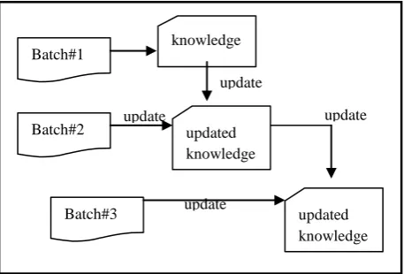
This scenario can be related to a distributed environment where knowledge merging is sequence optional but it is possible that the optimal way of merging might be sequence sensitive [11,14]. It is significant to note here that the nature of inflowing information could be naturally subsetted because features arrive in batches. Each batch can produce its own local knowledge. The cumulative knowledge from all batches can be obtained either in parallel or sequentially based on the domain knowledge.Figure 2. Features arriving in batches
Add features
Add features extract
Dimension ality Reduction
knowledge
Updated knowledge
Add features
update
Updated knowledge
extract Batch#1
Batch#2
Batch#3
knowledge
updated knowledge
updated knowledge update
update
update
3.3 Streaming of features from
multisensors
Tracking the pattern, reducing noise and narrowing down on the highly variant features [45] in practical applications such as radar, sonars etc can prove to be very useful. Each sensor will have its own domain in scope and the local knowledge derived out of each sensor can have significant information by themselves as well as the cumulative knowledge derived by incrementally reducing the features from all sensors. Let us consider receiving data from 2 sensors while waiting to receive data from the third sensor ( see Figure 3 ). To make the best possible decision, the local knowledge obtained by incrementally reducing the first 2 sensors can be used to arrive at the decision making parameters. One need not wait for the third sensor’s data to arrive to make a decision at this point, if necessary. When the third sensor streams data, one could update the knowledge by incrementally merging its local knowledge to the existing knowledge further bolstering the idea of capturing the most prominent features with maximum variance. A similar scenario can be seen in a LMS environment. When a class of students receive scores from 4 different courses of distinct disciplines representing different sensors, it can be related to the case of a constant sample space with varying feature space that collects information from different sensors. The local knowledge can be used for periodic feedback not only for students but also for teachers to evaluate and/or improve their pedagogical strategies.
Figure 3. Features streaming from multisensors
This can be a specific case of features arriving from different sources and the framework presented in this section also illustrates the possibility of arrival of multisensory data temporally.
3.4 Availability of all features together
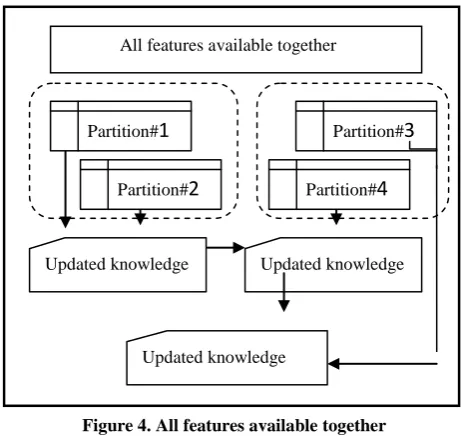
If climatic data for a duration of last 50 years has to be worked on to reduce the feature space, reducing it in one go might not be feasible. Smaller chunks of feature spaces can be partitioned and processed. Each partition can represent a single batch. To combine and/or merge the features optimally, many researchers have worked on several feature space partitioning methods which often involve clustering or classification of features [4, 6]. Research has shown that the simultaneous partitioning of the feature space and an assignment of a combined classifier to each of the subsets yields optimal feature space [37]. Given a set of n features, it can be partitioned into batches of features (see Figure 4) and each batch can inturn be worked upon to reduce the complexity of computation. This is analogous to parallel programming. In such cases the significance of incremental [image:3.595.313.544.137.360.2]knowledge is minimal because all the features are available to make a decision or to arrive at the decision making parameters. The challenge here will be to effectively partition the batches and merge the knowledge with minimum computation [11].
Figure 4. All features available together
4.
ILLUSTRATIVE EXPLORATION
In this paper, the objective of exploring the proposed incremental dimensionality reduction is to incrementally arrive at the reduced feature space and to accumulate the local knowledge so that the best decision making parameters at any instant of time can be availed. In general, at all times the exploration targets to achieve the following:
Selecting and retaining the best subset of features incrementally by eliminating redundant ones
Shifting the change in loci incrementally as per the feature changes in the arriving batches.
Maintaining and updating the cumulative knowledge derived out of the reduced feature space without looking back at the previous feature space
4.1 Simulation of big feature space through
exploitation of iris dataset
To begin with, the original Iris data set [46] of 4 features for Incremental reduction has been considered since it is a benchmark dataset. Though it is not a high dimensional dataset, Iris dataset is considered not only because it is an excellent benchmark for pattern recognition problems but it also serves the purpose of extrapolation as well. Extrapolation of features in a dataset extends the data while varying the variation in the feature space to be reduced. Similar effort has been made to illustrate dimensionality reduction in hyper spectral data [50]. Extrapolation is done by extending the corresponding values of the original feature set. To extend the values, different extrapolation methods like increasing the feature value by 10% or by decreasing by 5% etc have been used. A simple incremental feature subsetting procedure is conducted by employing Pearson’s correlation coefficient to define the threshold of elimination of features. This results in getting 2 features in the reduced feature space ie. sepal width and petal length that show the maximum variance. In order to illustrate the procedure on a bigger feature set, the original Iris features of 4 features are extract knowledge
updated knowledge Sensor
#1 #1 Sensor #2
#1 Sensor
#3 #1 update update
All features available together
Partition#
1
Partition#
2
Partition#4
Partition#3
Updated knowledge
[image:3.595.52.282.374.527.2]Volume 97– No.12, July 2014
extrapolated to 24 features represented by the alphabets B, C, D,..., P, Q, R,...and Y.
Many random combinations of features have been explored to understand how the proposed incremental dimensionality reduction works. To explain all the exhaustive combinations is not in the scope of this paper. So a good enough set of combinations are considered to illustrate the research proposal comprehensively. Let us consider a set of 24 features arriving in 6 batches. The derivation of incrementally reducing the feature space is illustrated as below. In real time scenario, most often, one cannot afford to wait for all the features to be available to make a decision. For example when information from two sensors is available and while waiting for the information from the third sensor to arrive, decisions have to be made. In such cases where real time decisions need to be taken as the locus changes, the highly variant feature subset can be incrementally derived. Such a subset can be used to analyse and provide sufficient knowledge for decision making at any instance of time. As the features arrive in batches, features with higher variation dominates the other features which have lesser variation.In other words, the features that encompass maximum variation survive feature elimination at every phase because the reduced feature space contains the maximum available information with less redundancy.
4.2 Usage of extrapolated iris data for
illustration of incremental feature
subsetting
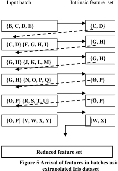
In the extrapolated Iris data example, let us assume that 6 batches of 4 features arrive in sequence : {B, C, D, E}, {F, G, H, I}, {J, K, L, M}, {N, O, P, Q},{R, S, T, U} and {V, W, X, Y} (see Figure 5) . As mentioned before the original set of 4 features {B, C, D, E} reduces to {C, D} in the first batch. In the next step, the reduced feature space {C, D} with the next batch of features {F, G, H, I} is merged and the feature subsetting algorithm is applied to arrive at an intrinsic subset {G, H}. Incrementally, reduced feature space containing features G and H are replaced by features O and P in the following step because the standard deviation of O and P are higher than G and H respectively. Subsequently, they are inturn replaced by W and X again due to higher standard deviation supporting the fact that the reduced feature space will always have the best possible maximum variance. It is interesting to gather that W and X are the corresponding extrapolated values of C and D which exhibit the most variance in the original Iris dataset of 4 features. Considering data coming in various batches, many combinations of features have been tried out with varying batches and number of features in batches. It is observed that in the extrapolated Iris data set, regardless of the sequence in which batches arrive, the incremental dimensionality reduction finally gives us the same feature subset {W, X}in the reduced feature space.
[image:4.595.313.509.73.356.2]
Figure 5 Arrival of features in batches using extrapolated Iris dataset
Another possibility with feature arrival could be when the feature batches of random length arrive. The merging and derivation of local knowledge becomes sequence compulsive in this case. If this scenario is simulated with the extrapolated Iris dataset, it is observed that the intrinsic knowledge being captured incrementally will be in the same way as when features arrive in batches. An exhaustive combination of batches is made to arrive in batches of random length and it is found that the final feature set remains the same i.e. {W, X} in all cases.
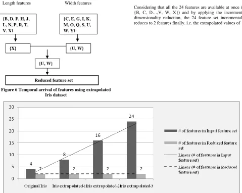
Next, the simulation of multisensor data using Extrapolated Iris data is explored. Let us consider all the ‘length’ related features {B, D, F, H, J, L, N, P, R, T, V, X} coming from one sensor and the ‘width’ related features {C, E, G, I, K, M, O, Q, S, U, W, Y} coming from another sensor (see Figure 6). Consider the first sensor as the first batch and the second sensor data as second batch and apply incremental dimensionality reduction. If the first batch is reduced alone, X is obtained in the reduced feature space and the second batch by itself reduces to {U, W} (see Figure 6). When X and {U, W} are incrementally reduced further , {U, W} emerges as the reduced feature set that cannot be reduced further. Since X and U are highly correlated and the standard deviation of U is higher than X, X gets eliminated retaining {U, W}. The reduction procedure reduces the extrapolated Iris feature set to the features {W, X} in the reduced feature set. It is important to observe here that although a different set of reduced space is obtained when the sequence of the feature arrival is changed, the incremental dimensionality reduction algorithm works towards retaining the maximum variance in order to capture more knowledge.
{G, H}
{G, H} {B, C, D, E}
{C, D} {F, G, H, I}
{G, H} {J, K, L, M}
{G, H} {N, O, P, Q}
{O, P} {R, S, T, U}
{O, P} {V, W, X, Y}
{C, D}
{O, P}
{O, P}
{W, X}
Reduced feature set
Figure 6 Temporal arrival of features using extrapolated Iris dataset
Considering that all the 24 features are available at once (ie {B, C, D…,V, W, X}) and by applying the incremental dimensionality reduction, the 24 feature set incrementally reduces to 2 features finally. i.e. the extrapolated values of
Figure 7. Trend of reduced feature set in extrapolated Iris data
Sepal Width and Petal Length {W, X}. Here the final reduced space contains the extrapolated values of the original features{C,D} because the standard deviation is higher in those than the original features .It is observed that the reduced feature space of extended data is in sync with the reduced feature space of the original data which further fortifies the incremental reduction procedure and its results. Iris dataset with 4 features was extrapolated to 8, 16 and 24 features and incrementally reduced separately (see Figure 7). When the number of features for input were increased gradually, the reduced feature set remained constant i.e. the reduced feature set always ended up with the same 2 features. At every step of the incremental reduction, the reduced feature space consists of the maximum available variance while moving towards accumulating the knowledge up to that level. It is important to observe that the updation of knowledge incrementally is also achieved without looking back at the previous feature space.
4.3
Algorithm development
Batches can be interpreted by the nature of flow of information. In temporal data a batch can arrive at different point in time, season or duration. In a distributed environment, batches can be coming from different sources. In either case each batch encapsulates its own local knowledge. The interest of the research proposal is to see
how the encapsulated knowledge can be accumulated. Having explored the various aspects of incremental dimensionality reduction, an algorithm is developed as below. The 2 important factors of this algorithm are Pearson’s correlation coefficient (r) and threshold factor (t).The measure of strength of correlation between 2 features is given by ‘r’. Threshold factor ‘t’ is the cutoff value to determine whether the features are related close enough to be considered for elimination. When the Iris dataset was considered to obtain ‘t’ by trial and error method, for t= 0.65, the correlation was very strong and would leave some of the closely related features in the reduced space increasing redundancy. At t=0.55, the correlation was not good enough to be considered for elimination due to considerable variance among the features. The ideal value t =0.6 was determined by trial and error method that would distinctively differentiate the features for elimination and also aid in arriving at the optimal feature subset. Adding to this, exhaustive incremental dimensionality reduction has been conducted on datasets like extrapolated Iris dataset, Corn Soya [47,48], Wine data sets [49] and found that the threshold at 0.6 provided consistent results supporting the threshold value substantially. Subsequently, the algorithm was arrived at as below:
Input: A set of features of the original dataset DB
{C, E, G, I, K, M, O, Q, S, U, W, Y} {B, D, F, H, J,
L, N, P, R, T, V, X}
{U, W} {X}
{U, W}
Reduced feature set
Volume 97– No.12, July 2014
B= {F0, F1, F2,…, FN} where B is a batch of features
Output: Reduced feature set of the original dataset DB
I= {f0, f1, f2 …, fn} where I is the reduced feature set Consider n features with k batches
Begin
Initialize the intrinsic feature subset to an empty set. While number of input batches >=1 Do
1. Generate all possible combinations of 2 features of the batch with n features C (n, 2)
2. Calculate Pearson’s coefficient(r) for each pair of features 3. For each pair of features
If (r>=threshold) Then
Add the feature that has a higher standard deviation to the intrinsic feature subset. Else
Add both the features to the intrinsic feature subset I which constitutes the reduced feature space at that instant
EndIf Loop
4. Merge the intrinsic feature subset ‘I ‘ with the next batch of features
// Repeat 2-4 until there are no more input batches End Do
End
The Intrinsic feature subset ‘I’ now has the most reduced feature set of DB that cannot be reduced further
The best case scenario is when there are only 2 features. The reduced feature space can be obtained in kC2 =1 where k (# of batches) =1
tΩ Ω (1)
The worst case scenario is when there is maximum number of k features. All possible combinations will be computed k!/((k-2)! * 2!) ) times. So,
t(O) O(k!/2)) where k>2
5.
EXPERIMENTAL ANALYSIS
Iris dataset and the extrapolated Iris datasets were used earlier to illustrate and explore the aspects of incremental dimensionality reduction. Multivariate dataset like wine dataset [49] has been used to analyze the incremental dimensionality reduction while observing the flow of
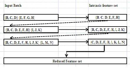
features to confer with the analysis derived from the extrapolated Iris dataset. Wine dataset is the result of chemical analysis that can determine the origin of wines. Original wine dataset has 13 features represented by the alphabets B, C, D……. L, M and N. For illustration (see Figure 8), let us consider the 13 features arriving in 4 batches: {B, C, D} , {E, F, G, H} , { I, J, K} and {L, M, N}.
Figure 8 Arrival of features in batches using wine Dataset
When incremental dimensionality reduction is applied to the first 2 batches , only one feature ‘G’ is eliminated due to the high correlation of feature G among the other features. The reduced feature space at this point consists of {B,C,D,E,F,H} which represents the local intrinsic knowledge that is in turn considered as another batch to merge with the second batch {I, J, K}. By repeating this procedure until the batches exhaust, the final reduced feature set obtained is {C, D, E, F, H, I, K, L, N} (see Figure 8). Here again one can observe that the same reduced feature set {C, D, E, F, H, I, K, L, N} is obtained irrespective of the sequence of batches; bolstering the fact that incremental dimensionality reduction need not be sequence compulsive. Among the 13 attributes, 9 attributes (malic acid, ash, alkalinity of ash, magnesium, flavanoids, nonflavanoid phenols, color intensity, hue and proline represented by C, D, E, F, H, I, K, L and N respectively) from the reduced feature space encapsulates the maximum variance of the wine dataset that can be used to determine the origin of wine. These 9 attributes can be assigned higher weightage during classification as they will constitute towards stronger decision making parameters. The other 4 attributes ( alcohol, total phenols, Proanthocyanins and OD280/OD315 of diluted wines represented by B, G, J and M respectively) have a higher correlation in the dataset. So the 4 attributes can be assigned a lesser weightage as they might not significantly contribute towards decision making during incremental learning.
5.1 Dimensionality reduction of the
temporal corn soya dataset
[image:6.595.320.541.155.275.2]batch is merged to reduce it further. The reduced feature space now has {F,K} that is merged with the July batch to get {F,Q} in the reduced space. The incremental procedure is followed until the last batch from August is merged with the reduced feature set of the other three previous batches to obtain { F,Q,W} in the feature space that cannot be reduced any further. It is observed that as the new batch arrives temporally, the feature ‘F’ with the maximum variation incrementally dominates while eliminating the redundant features. As the incremental feature subsetting takes place, the knowledge available for prediction at any given instance of time also adapts accordingly while improving the accuracy of classification,
Figure 9. Converging towards an optimal feature subset in temporal Corn Soya data
5.2 Evaluation of Classification while
converging towards an optimal feature
subset
As the features get reduced incrementally, the relevance of the features in the feature set is analyzed by using the metrics to evaluate the classification accuracy. The performance of classification can be evaluated using metrics like precision, recall and accuracy. The accuracy is the proportion of the total number of predictions that were correct. The recall or true positive rate is the proportion of positive cases that were correctly identified and precision is the proportion of the predicted positive cases that were correct [51].
[image:7.595.55.289.227.369.2]At each intrinsic feature set, the classification accuracy was analyzed by using these metrics to understand how the accuracy works along with incremental dimensionality reduction.
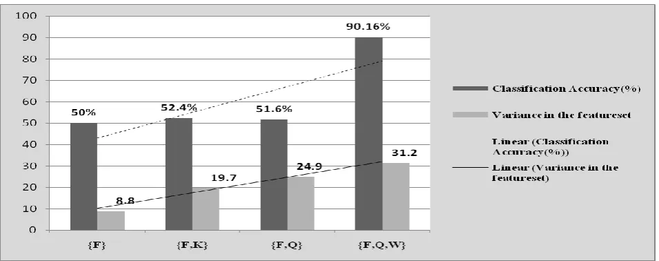
Table 1. Classification Evaluation of Corn Soya dataset
Metric/Intrinsic feature set
{F} {F,K} {F,Q) {F,Q,W}
Precision 50 51.2 50.8 83.56
Recall 100 100 100 100
Accuracy 50 52.4 51.6 90.16
Variance 8.8 19.7 24.9 31.2
As Corn Soya data arrives temporally, the reduced space follows an incremental pattern (Table. 1) i.e. {F} {F, K} {F, Q} {F, Q, W} ( see Figure 9). The first batch of features (i.e. Jun 11) identify and retain {F} as the feature with the most variance. For the Jun 11 batch, Accuracy of Classification is 50% meaning that feature F at this phase can positively predict the classes 50 % of the time helping in narrowing down on the most prominent feature at that particular phase. Moving to the next batch of features (i.e. Jun29), the algorithm retains F and adds K to the reduced space. Here, the accuracy improves to 52.4%.
Moving forward, the incremental dimensionality reduction algorithm reduces the feature subset {F,K} to {F,Q} when July set arrives, the classification accuracy slows down with a minor difference in the classifier performance but retains the maximum variation in the reduced feature space. Also one can observe that feature F remains as a dominating feature that consistently survives every phase of elimination. The Pearson’s correlation coefficient(r) of {K, Q} = 0.68. When r >0.6 , the classifier performance will not make a significant difference incrementally due to higher correlation of the attributes but certainly maximizes the variation of the feature subset .i.e. the algorithm continues to increase the maximum variance in the feature set (see Figure 10). The standard deviation of feature K is less than that of feature Q.
[image:7.595.55.533.545.734.2]Volume 97– No.12, July 2014
So the incremental dimensionality reduction retains Q while eliminating K . As it further progresses to incrementally incorporate the August month changes , it retains the features that have the maximum variation {F,Q},adds another feature {W} that brings a significant improvement in classification Accuracy of 90.16%. So at any given instant of time during the lifetime of the reduced feature space , the best reduced feature set can be made available for decision making without waiting for the entire feature set to arrive and without looking back at the previous feature space.
5.3 Validation of the proposed incremental
learning
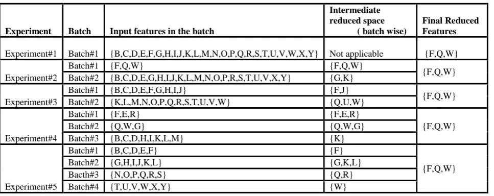
Although Corn Soya is a temporal data set, let us consider that all the features become available together and apply the proposed incremental dimensionality reduction procedure. Experiment#1 is a case where all the features are available at once. The reduction procedure results in the reduced space { F, Q, W}. To validate if the final reduced space is the same as the one that is achieved while applying the proposed incremental reduction , we consider various combination of batches from Corn Soya dataset ( see Table 2). A significant
number of experiments were carried out to analyze the proposed incremental dimensionality reduction. For the purpose of illustration , only a handful of the experiments carried out using Corn Soya data are listed (see Table 2). For experiment#2 to experiment #5, the incremental dimensionality reduction yielded the same reduced feature set i.e. {F, Q, W} . If the features with maximum variance i.e. {F,Q,W} are made to arrive in first or middle or the last in the sequence of batches , the reduction algorithm will give back the same subset {F,Q,W} as the reduced feature set that gives the highest classification accuracy. At all times during the incremental reduction, the procedure ensures that the knowledge in the form of maximum variance is carried forward to the next phase .
[image:8.595.49.533.322.514.2]Regardless of the order in which the features arrive, the algorithm consistently captures the maximum variance which bolsters the proposed idea that the best available feature space can be extracted even at an interim phase and it can be utilized for further prediction and/or analysis (see Table 2). Similarly the Corn soya data is simulated to arrive from different sensors by splitting them into n number of batches [47].
Table 2. Consistency of arriving at the reduced feature space incrementally
For all the experiments that were carried out , the proposed incremental dimensionality reduction consistently resulted in the same reduced feature space. Whether the data is streaming, temporal or coming from multisensors, incremental dimensionality reduction works consistently in containing the knowledge without the need to look back at the previous feature space.
6.
CONCLUSION AND FUTURE
WORK
Incremental Dimensionality reduction has the ability to adjust the locus change as the context of the feature space changes and to capture the local knowledge which is most often not possible with the conventional dimensionality reduction. At every phase of reduction, the maximum variation available that best describes the original feature set is incrementally obtained, thus projecting the most prominent feature/feature set at every step for analysis or decision making or prediction. Incremental dimensionality reduction handles variance in such a way that it shows consistency in capturing the local knowledge at every phase of reduction without looking back at the old data for deduction. One need
not wait for all the sources to provide information before making the best possible decision because the parameters available at an interim phase will be converging towards the final solution.
The results of incremental dimensionality reduction can be utilized for making decision at any given point in time based on the local knowledge at every phase regardless of its distributed origin or a temporal viewpoint. The order of arrival of features does not significantly alter the spread of variation in the finally reduced feature space. The most dominant feature that shows the maximum variance in the reduced feature space stands out at every phase which emphasizes its variation in the reduced feature space. The most dominant feature by itself might not be the best classifier but it will be a part of the best classifier when the cumulative feature space displays the maximum variance. It is observed that by cumulatively holding on to only the features that would matter in future, looking back at the previous data to capture the most effective knowledge at a given instant can be avoided.
Experiment Batch Input features in the batch
Intermediate reduced space ( batch wise)
Final Reduced Features
Experiment#1 Batch#1 {B,C,D,E,F,G,H,I,J,K,L,M,N,O,P,Q,R,S,T,U,V,W,X,Y} Not applicable {F,Q,W}
Experiment#2
Batch#1 {F,Q,W} {F,Q,W}
{F,Q,W} Batch#2 {B,C,D,E,G,H,I,J,K,L,M,N,O,P,R,S,T,U,V,X,Y} {G,K}
Experiment#3
Batch#1 {B,C,D,E,F,G,H,I,J} {F,J}
{F,Q,W}
Batch#2 {K,L,M,N,O,P,Q,R,S,T,U,V,W} {Q,U,W}
Experiment#4
Batch#1 {F,E,R} {F,E,R}
{F,Q,W}
Batch#2 {Q,W,G} {Q,W,G}
Batch#3 {B,C,D,H,I,K,L,M} {K}
Experiment#5
Batch#1 {B,C,D,E,F} {F}
{F,Q,W}
Batch#2 {G,H,I,J,K,L} {G,K,L}
Bacth#3 {N,O,P,Q,R,S} {Q,R}
Incremental dimensionality reduction can be used to incrementally derive the knowledge in the transformed feature space as well while observing the nature of incremental flow of features. It can be further explored on the possibility of incremental updation of knowledge in terms of original features which are engulfed in the transformed and reduced feature space. Working with transformed feature space might not be as transparent as working with feature subsetting because feature transformation assimilates the knowledge in the reduced feature space. This would make it even more challenging to incrementally discover the knowledge in a transformed feature space.
7.
REFERENCES
[1] Edilson Delgado-Trejos et,al, Dimensionality Reduction Oriented Toward the Feature Visualization for Ischemia Detection, IEEE Transactions on Information Technology in BioMedicine, Vol13, No04, 2009. [2] Chowdhury.F et, al, Single-pass incremental and
interactive mining for weighted frequent patterns, 2012. [3] J. Han, M. Kamber, “Data Mining: Concepts and
Techniques,” Third Edition, Elsevier Inc., Rajkamal Electric Press, 2011.
[4] S. Santhosh Kumar et,al "Development of an Efficient Clustering Technique for Colon Dataset" IJEIT, Vol1, Issue 5, May 2012.
[5] Bing Lu., Wynne Hsu., Yiming Ma, Integrating Classification and Association Rule Mining, KDD proceeding AAAI, 1998.
[6] Francesco Palumbo., Alfonso Iodice D’Enza, Clustering and Dimensionality Reduction to discover interesting patterns in Binary data, Proceedings of the 32nd Annual Conference of the Gesellschaft für Klassifikation e.V., 2008
[7] P.Adraig Cunningham, Dimension Reduction ,Machine Learning Techniques for Multimedia Cognitive Technologies , pp 91-112, 2008
[8] Francesco Palumbo., Alfonso Iodice D’Enza, Clustering and Dimensionality Reduction to discover interesting patterns in Binary data, Proceedings of the 32nd Annual Conference of the Gesellschaft für Klassifikation e.V., 2008
[9] http://en.wikipedia.org/wiki/Dimensionality_reduction [10]
http://www.cs.binghamton.edu/~lyu/SDM07/DR-SDM07.pdf
[11] Syed Zakir Ali., P Nagabhushan., Pradeep Kumar R, Incremental datamining using Clustering Intelligent methods of Fusing the Knowledge During Incremental Learning via Clustering in A Distributed Environment , PhD Thesis, 2010
[12] J.Bailey , E.Loekito,Efficient incremental mining of contrast patterns in changing data, 2010.
[13] T.Gharib et,al, An efficient algorithm for incremental mining of temporal association rules, 2010.
[14] Syed Zakir Ali., P Nagabhushan., Pradeep Kumar R, Regression based Incremental Learning through Cluster Analysis of Temporal data, International Conference on Data Mining (DMIN) 2009.
[15] D.Dudek, RMAIN:Association rules maintenance without reruns through data, 2009.
[16] C.Hsu., Y.Huang. Incremental Clustering of mixed databased on distance hierarchy, 2008
[17] F.Masseglia., P.Poncelet., M.Teisseire, Incremental mining of sequential patterns in large databases, 2003. [18] Zhang.M et,al, Efficient algorithms for incremental
update of frequent sequences, 2002.
[19] N. Sarda, N.V. Srinivas, An adaptive algorithm for incremental mining of association rules, in: Proceedings of the 9th International Workshop on Database and Expert Systems Applications, Indian Institute of Technology, Bombay, 1998
[20] Jieping Ye., IDR/QR: an incremental dimension reduction algorithm via QR decomposition, Knowledge and Data Engineering, IEEE Transactions , Vol17, Issue09, 2005
[21] Martin H.C. Law, Anil K. Jain, Incremental Nonlinear Dimensionality Reduction by Manifold Learning, IEEE Transactions on Pattern Analysis and Machine Intelligence, vol. 28, no. 3,2006
[22] Sheng Uei Guan et al., Incremental Learning with Respect to New Incoming Input Features, Neural Processing Letters 14, 2001
[23] Courses.cs.tamu.edu/rgutier/cs790_w02/l5.pdf – United States
[24] http://dss.princeton.edu/training
[25] Guan SU, Li S, Incremental learning with respect to new incoming input attributes, Neural Processing Letters 14(3):241–260,2001
[26] T. Wang and S. U. Guan, “Feature ordering for neural incremental attribute learning based on Fisher's linear discriminant,” in Proceedings of the 5th International Conference on Intelligent Human-Machine Systems and Cybernetics (IHMSC '13), Hangzhou, China, 2013 [27] Murat Karabatak et,al, A new feature selection method
based on association rules for diagnosis of erythemato-squamous diseases, Expert Systems with Applications, Vol36, Issue10, 2009
[28] Hua-Liang Wei., Billings.S.A, Feature Subset Selection and Ranking for Data Dimensionality Reduction, Pattern Analysis and Machine Intelligence, IEEE Transactions, Vol 29, Issue01, 2007
[29] Bartosz Krawczyk., Pawel Filipczuk., Michal Wozniak, Adaptive Splitting and Selection Algorithm for Classification of Breast Cytology Images. ICCCI (1), 2012.
[30] Gulsen Taskin Kaya et.al, Feature selection by high dimensional model representation and its application to remote sensing Geoscience and Remote Sensing Symposium (IGARSS), IEEE International, 2012 [31] http://www.ime.unicamp.br/~wanderson/Artigos/feature
_selection_in_mining.pdf
Volume 97– No.12, July 2014
[33] Liu.,Yu, Toward Integrating feature selection algorithms for classification and clustering, Journal of Knowledge and data engineering, Vol17,Issue04 [34] Tin Wang, Feature Ordering for Neural Incremental
Attribute Learning Based on Fisher's Linear Discriminant (Intelligent Human- Machine Systems and Cybernetics (IHMSC), 5th International Conference on vol2, 2013
[35] Huan Liu et al.,Incremental Feature selection, Journal Applied Intelligence, Vol 9 Issue 3 ,pp 217-230, 1998 [36] Michal WozNiak., Bartosz Krawcztk, Combined
Classifier based on Feature space partitioning, Int. J. Appl. Math.Comput. Sci.,Vol22, No04, 2012.
[37] S. Kotsiantis., K. Patriarcheas., and M. Xenos. A combinational incremental ensemble of classifiers as a technique for predicting students’ performance in distance education, 2010.
[38] D. Brauckho et al., Anomaly extraction in backbone networks using association rules ,In Proceedings. of IMC, 2009.
[39] Murat Karabatak ,M. CevdetInce An expert system for detection of breast cancer based on association rules And neural network, journal, Expert Systems with Applications 36(2009) 3465–3469, 2009.
[40] Agrawal, H. Mannila, R. Srikant, H. Toivonen, and A. Verkamo. Fast discovery of association rules. In U. Fayyad, G. Piatetsky-Shapiro, P. Smith, and R. Uthurusamy, editors, Advances in Knowledge Discovery and Data Mining, pages 307-328. AAAI/MIT Press, 1996
[41] Minyoung Kin., Correlation-based incremental visual tracking, The Journal of the Pattern Recognition Society, Vol45, Issue03, 2012
[42] Flip Korn et al., Quantifiable datamining using PCA, VLDB Journal: Very Large Data Bases, 1997
[43] Anil K. Jain's talk: Clustering Big Data, University of Notre Dame, Nov. 29, 2012
[44] http://www.coffeechoiceguide.co.uk/coffee-regions.htm [45] http://www.fusion2014.org/tutorials/t14-mtpa
[46] Yates, F.; Mather, K., "Ronald Aylmer Fisher 1890-1962". Biographical Memoirs of Fellows of the Royal Society 9: 91–129,1963.
[47] P. Nagabhushan, An efficient method for classifying remotely sensed data (incorporating dimensionality reduction), Ph.D thesis, Universityof Mysore, 1988 [48] Rangarajan, Lalitha, and P. Nagabhushan.
"Dimensionality reduction of multidimensional temporal data through regression." Pattern recognition letters 25.8 (2004): 899-910.
[49] http://archive.ics.uci.edu/ml/
[50] P.Nagabhushan, H.N.Meenakshi.,"Target Class Supervised Feature Subsetting", International Journal of Computer Applications,Volume 91, Issue12, 2014 [51] http://www2.cs.uregina.ca/~dbd/cs831/notes/confusion_