Software Project Scheduling by AGA
Dinesh Bhagwan Hanchate
Comp. Engg. Deptt. V.P.’s College Of Engg.,Baramati, Pune
Rajankumar S. Bichkar
Prof. ( E & Tc ) and Dean G. H. R. C. O. E. M., Wagholi,Pune, India.
ABSTRACT
This paper proposes general techniques for adapting operators in SGA for software project scheduling problem. The use of adap-tive of crossover and mutation gives chance to control the diver-sity. Adaptive nature also tends to give convergence in the com-plex solution. Crossover and Mutation probability changes ac-cordingly the change in the fitness values. High fitter is kept in the next pool. AGA(Adaptive genetic algorithm) converges to sub-optimal solution in fewer generation than SGA. In this pa-per, we consider skilled employees as an important resource to calculate the cost of the project along with some constrains of tasks. The paper gives a near-optimal estimated cost of project by using AGA. Our algorithm employs adaptive approaches for calculation of fitness of individuals, crossover rate and mutation rate. The paper also considers the aspects of head count, effort and duration calculated by COCOMO-II.1999. These parameters are used to verify the fitness of each chromosome to get esti-mated cost by AGA closer to the cost estiesti-mated by COCOMO-II.
General Terms:
Software Project Management, Machine learning
Keywords:
AGA, COCOMO-II, Software Cost Estimation, Project Schedul-ing.
1. INTRODUCTION
1.1 Natural evolution and GA
Natural evolution is discussed and expressed by one of its first pro-ponents, Charles Darwin. His theory of evolution was based on four primary axioms [12].
?An offspring has many of the characteristics of its parents. This axiom implies that the population is stable.
?There are variations in characteristics between individuals that can be passed from one generation to the next.
?The third axiom is the only a small percentage of the offspring produced survive to adulthood.
?Survival of offspring depends on their inherited characteristics. These all axioms and presumptions together imparts the theory of natural selection.
Another set of biologically-inspired methods are Genetic Algo-rithms (GAs). They derive their inspiration from combining the
concept of genetic recombination with the theory of evolution and survival of the fittest members of a population [7]. The learning process devises better and better approximations to the optimal pa-rameters, starting from a random set of candidate parameters. The GA is primarily a search and optimization technique. The genetic algorithm is a one of the family of evolutionary algorithms. Darwin discovered that species evolution based on two components: the se-lection and reproduction. The sese-lection provides a reproduction of the strongest and more robust individuals, while the reproduction is a phase in which the evolution run.
The behavior of the GA depends on how we get the values of pc and pm. There are a various ways being told in regarding choos-ing pc and pm, by K. A. DeJong [25] [18].These are inadequate as the choice of the optimal pc, and pmbecomes specific to the software problem under consideration. Grefenstette has formulated the problem of selecting pcand pm, as an optimization problem in itself.A theoretical comparison of randomized and genetic op-timization algorithms concluded that many GAs are characterized by higher probability of finding good solutions than randomized al-gorithms, as long as the solution space fulfills several restrictions. These restrictions however are weak and hold for almost any choice of the genetic operators [13].
It is important to prevent promising individuals from being elim-inated from the population during the application of genetic op-erators. To ensure that, the best chromosome is preserved, elitist methods copy the best individual found so far into the new popula-tion [25] [46]. However, elitist strategies tend to make the search more exploitative rather than explorative and may not work for problems in which one is required to find multiple optimal solu-tions [46]. In elitist strategy, the offspring have to compete with the parents to gain admission for next generation of GA [52]. The outstanding advantage of this environment is it always preserve the best solutions in every generation. Discussions on exploitation and exploration trade-off (by F. van den Bergh) has initiated the idea to investigate tournament and roulette wheel schemes other than deterministic in elitism strategy.
1.2 Related work
The approaches to project scheduling can be summarized as fol-lows:
neural networks), and hybrid systems.
The scheduling problem is usually described as the task of integer programming. In such tasks, the vector of decision variables usu-ally takes the form of a binary vector Brucker et al. 1999; Kasprow-icz 2002; Kolish and Padman 1997; Marcinkowski 1990; Weglarz 1981. Precise procedures of single-criterion optimization of sched-ules are mainly based on the branch and bound method Dorndorf et al. 2000; Kasprowicz 2002; Weglarz 1981. To solve serious practi-cal problems using precise algorithms is impossible because of the length of time needed for the calculations and the limited memory capacity of computers Marcinkowski 1990; Slowinski et al. 1994; Weglarz 1981.
Thus several approximation methods employing the heuristic ap-proach have been conceived. The methods can be divided into two groups: specialized heuristics and meta-heuristics. Specialized heuristics can be used to solve only one optimization problem. Priority heuristics is among the most well known heuristics solv-ing schedulsolv-ing problems which is usually available in the project scheduling software. Priority heuristics are of two phases. The first phase prepares and arranges priority lists of processes according to decreasing values of priorities. The second phase calculate the start and finish times of these processes so as to keep to all the con-straints in. In this phase, one of the two methods of tasks schedul-ing is used: parallel or serial, which differ in how they solve re-sources conflicts. The second phase is considered in our approach to have parallel tasks which are independent with each others. The works of Shanmuganayagam in 1989, Tsai and Chiu in 1996, and Ulusoy and zdamar in 1995 uses priority heuristics for scheduling projects and resources allocation. We used priority scheduling with respect to TPG only. Priority schedule may reduce the results that’ why Khamooshi in 1996 modified the existing approach to estab-lish process priorities. The procedure Khamooshi worked out and in dividing a project into parts and using a different priority rule for each part. He presents this approach in the form of a dynamic programming model. Slowinski et al. 1994 suggested employing a cluster of many rules instead of one priority rule, and then choos-ing the best one. We clustered the rules in terms of Hard and Soft constraints in our approach. To solve single-criterion optimization problems in scheduling projects, metaheuristic algorithms can also be used. They define only a certain pattern of optimization proce-dure, which must be adapted for particular applications software project scheduling by ACO (Jing Xiao, Xian-TingAo, YongTang 2012).
The most frequently used metaheuristic methods are taboo search, simulated annealing, and evolutionary algorithms. Actually, Neigh-borhood local search algorithms include simulated annealing and taboo search method ( Sampson and Weiss 1993). They searched the feasible area solutions going from a current solution to a neigh-boring one. The natural imitating processes used in local search methods are also used in evolutionary algorithms.
1.3 Concerned readings and inspiration
The work done in fields, domains and sub-domains produced in various related papers are significantly carried out by some mean of related areas like genetics, GA, adaptiveness, software engineering, data structure required for GA, project management and interdisciplinary work done by researchers and authors. The readings of all the following papers is done for doing the study of various angles in the proposed approach. The work done by Mark [31], Dark [10], Sahani [22], Uyar [44], Forest [35], Imtiaz [24], Hayenes [20],Fogarty [16], Back [2], Yang [45], Therens [51] [50], Macheal and Shurva [?], Alba [14], Pinedo [41],
Tom [37], Keightley [27], Charles [3], Parag [39], Thorat and Am-bole [1], Zhang [57], Futuyam [17] and Jurgen [21].
1.4 Evolutionary algorithms
Evolutionary algorithms are classified into include evolution strate-gies, classifier systems,genetic algorithms, evolutionary program-ming, genetic programming.The results of research in this field are usually not classified according to an individual method but are generally described as evolutionary algorithms (Michalewicz 1996). Evolutionary algorithms work as computer systems for solv-ing problems accordsolv-ing to the rules observed in the evolution of live organisms. The rules involve system structure and the organisms ways function and adapt to existing conditions. A feature of this ap-proach to solving optimization problems is creating a population of individuals representing solutions in a form of a chromosome. As in nature, better-adapted individuals more effective solutions which stand a better chance of survival and development.
The evolutionary algorithms are used to solve optimization prob-lems in many branches of industry. A number of examples of their application, such as
]software project scheduling on timeliness GA (Carl chang 2010).
]basis the optimization of structures ( Koumousis and Georgiou 1994), engineering and design (Grierson and Pack 1993),
]selection of equipment for earth-moving operations (Haidar et al. 1999).
Some studies show that evolutionary algorithms have a consid-erable potential to solve many project scheduling problems effi-ciently.]For e.g., Li (1997;1999) used genetic algorithms to facil-itate the time-cost optimization, and Hegazy 1999 applies them to the optimization of resource allocation and leveling.
]Leu and Yang 1999 developed a multi-criteria optimization model for construction scheduling based on a genetic algorithm, which in-tegrates the time-cost trade-off model, the resource-limited model, and the resource-leveling model.
Some authors such as Padman 1997; Michalewicz 1996 classified evolution algorithms based on AI. Some experts like Adeli and Karim 1997, Kanet and Adelsberger 1987 solved the scheduling problem from ANN, expert systems apart from evolutionary algo-rithms.
Carl Chang proposed a tracking mechanism in the SPMNet [6]. He kept track of all the events through SDLC. An automatic technique based on genetic algorithms was introduced to determine the op-timal resource allocation in 1994 by him. He and their co-authors calculated the total time and cost of a project dependant on the information generated from GA. SM (Software manager) may be able to predict the future states of a project. Runwei CHENG and Mitsuo GEN (1994) suggested approach wich can significantly im-prove the performance of evolution program both in term of the speed and the accuracy. Marek Pawlak (1995) presented an evo-lution program for project planning to implement an optimisation resource demand. The GA simulation based approach was demon-strated by Julia Pet (1995) with stochastic task durations using a multiple RCPS (resource constrained project scheduling) problem .
evo-lutionary algorithms may be easily adapted to solving any type of problems, the proposed AGA method is versatile and allows defin-ing the case conditions and constraints freely [29].
In order to adjust a genetic algorithm [34] to the optimization problem it tackles, some kind of parameter control is usually em-ployed [33]. Adaptive control [26] uses feedback from the search to determine how the parameter values are to be altered. Self-adaptive control [?], puts additional information into the representation in order to provide some guidance to the operators. To date, most efforts on parameter control focused on adapting only one aspect of the algorithm at a time. The most comprehensive combination of forms of control [33] was offered in, where the adaptation of mutation probability, crossover rate and population size were com-bined. Other forms of adaptive systems for genetic algorithms can be found in [28] [36] . We proposed here a adaptive of a genetic algorithm which is able to dynamically adapt both the rate and the behavior for each of its operators.
All Genetic algorithms are a classified into stochastic type of op-timization methods inspired by the principles of natural evolution. The promising research area in this area is adaptation of strategy parameters and genetic operators. For getting optimum solutions, different adaptive techniques has been used to guide search of GAs. A key component of GAs is mutation which is a variable GA op-erator to create diversity in GAs. There are several adaptive muta-tion operators in GAs, including populamuta-tion level adaptive mutamuta-tion operators and gene level adaptive mutation operators. The experi-mental results of [24] show that the gene level adaptive mutation operators are usually efficient than the population level adaptive mutation operation.
The operator adaptation techniques in GAs can be classified into three categories, i.e., population level, individual level, and compo-nent level adaptation [40]. Operator adaptation depends on how op-erators are updated. At the population level, parameters are adapted globally by using the feedback information from the current pop-ulation. Individual level adaptation changes parameters for each individual in the population. Component level adaptation is done separately on some components or genes of an individual in the population [40].
Adaptation of strategy parameters and genetic operators has be-come an important and promising area of research on GAs. Many researchers are focusing on solving optimization problems by us-ing adaptive techniques, e.g., probability matchus-ing, adaptive pur-suit method, numerical optimization, and graph coloring algo-rithms [49, 52, 38]. The value of parameters and genetic operators are adjusted in GAs. Parameter setting and adaptation in mutation was first introduced in evolutionary strategies [47]. The classifica-tion of parameter settings has been introduced differently by the researchers [11, 48]. Basically, there are two main type of param-eter settings: paramparam-eter tuning and paramparam-eter control. Paramparam-eter tuning means to set the suitable parameters before the run of al-gorithms and the parameters remain constant during the execution of algorithms.Parameter control means to assign initial values to parameters and then these values adaptively change during the ex-ecution of algorithms.According to [11], parameters are adapted according to one of three methods: deterministic adaptation adjusts the values of parameters according to some deterministic rule with-out using any feedback information from the search space; adaptive adaptation modifies the parameters using the feedback information from the search space; and self-adaptive adaptation adapts the pa-rameters by the GA itself.
There are two main groups of adaptive mutation operators, one group are the population-level adaptive mutation (PLAM) opera-tors and the other are the gene-level adaptive mutation (GLAM)
[image:3.595.353.522.121.168.2]operators. Many researchers have suggested different static muta-tion probabilities for GAs. These static mutamuta-tion probabilities are derived from experience or by trial-and-error.
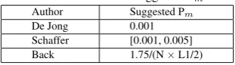
Table 1. Athours and suggested Pm. Author Suggested Pm
De Jong 0.001
Schaffer [0.001, 0.005] Back 1.75/(N×L1/2)
where, N means the population size and L denotes the length of individuals. This equation is based on Schaffers results [?]. In [11], it is suggested that Pm= 1/L should be generally optimal. It is very difficult, though not impossible, to find an appropriate parameter setting for Pmfor the optimal performance.
In the simple GA, the penalty function that is used to convert the constraints problems to unconstraint ones, and genetic operators, such as cross-over, mutation, and elitism, so on that are used to ex-plore the important regions of the search space are adopted. Since there is not a unique way to define the penalty scheme and genetic operators, different forms of these are proposed (Rajeev and Kr-ishnamoorthy, 1994; Rajan, 1995; Krishnamoorthy et al., 2002). In contrast to classical penalty scheme and genetic operators having the values of the various coefficients treated as pre-defined con-stants during the calculation of penalty function, some enhance-ments in the GA have been made and proposed by the researchers (Nanakorn and Meesomklin, 2000; Chen and Rajan, 2000; Srinivas and Patnaik, 2000; Togan and Daloglu, 2006 ) in order to increase the efficiency, reliability and accuracy of the methodology for code-based design of structures.
In this paper, adaptive approaches are proposed for both the penalty function and crossover and mutation probabilities in order to relieve the user from determining any values that are needed prior the op-timization and enhance the performance of the GA in optimizing SPSP. In the simple GA, the penalty function that is used to convert the constraints problems to unconstraint ones, and genetic opera-tors, such as cross-over, mutation, and elitism, so on that are used to explore the important regions of the search space are adopted. Since there is not a unique way to define the penalty scheme and genetic operators, different forms of penalty scheme and genetic operators are proposed (Rajeev and Krishnamoorthy, 1994; Rajan, 1995; Kr-ishnamoorthy et al., 2002). In contrast to classical penalty scheme and genetic operators having the values of the various coefficients treated as pre-defined constants during the calculation of penalty function, some enhancements in the GA have been made and pro-posed by the researchers (Nanakorn and Meesomklin, 2000; Chen and Rajan, 2000; Srinivas and Patnaik, 2000; Togan and Daloglu, 2006) in order to increase the efficiency, reliability and accuracy of the methodology used.In 1975, Holand ,De Jong, and in 1987 Ack-ley proposed one-point, N-point crossover and uniform crossover respectively.
The paper’s outline is organized as follows.
◦Section I, we discussed the GA & optimization, and the various techniques proposed in the literature and related work to overcome the problems.
◦Section II describes GA and it´s significance in optimisation.
◦In section III,We light on the role of project manager, importance of time management in SPM.
◦In section IV, we gave the utilisation of SEE (Software Engineer-ing Economics) in our approach.
◦In Section VI, our approach of using adaptively varying probabil-ities of crossover and mutation for SPSP (software project schedul-ing problem) is focused.
◦In section VII, We have Operations, Mathematical Modeling And Adaptive Fitness for our approach.
◦We illustrated input and output to our problem in section VIII.
◦A discussion of results obtained, some conclusions of the study and future work still to be done are explained in section IX,X,XI respectively.
2. GENETIC ALGORITHM
All GAs are inspired by the biological evolution. Each individ-ual represents binary strip called chromosome. Each element in the strip is called as gene where each individual shows the possi-ble solution of CO (Constraints optimization) propossi-blem in our hand after evolution. GAs are powerful methods of optimization used successfully in different problems. Their performance is depend-ing on the encoddepend-ing scheme and the choice of genetic operators especially, the selection, crossover and mutation operators. A va-riety of these latest operators have been suggested in the previous researches. In particular, several crossover operators have been de-veloped and adapted to the permutation presentations that can be used in a large variety of combinatorial optimization problems. Genetic algorithms (GAs) are powerful search methods. GAs were first introduced by John Holland in 1960s in USA. Nowadays,GAs have been successfully applied for solving many optimization prob-lems due to the properties of easy-to-use and robustness for find-ing good solutions to difficult problems [6]. The efficiency of GAs depends on many parameters, such as the initial population, the representation of individuals, the selection strategy, and the recom-bination (crossover and mutation) operators. Mutation is used to maintain the diversity of the entire population by changing individ-uals bit by bit with a small probability pm. Usually, the mutation probability has a significant effect on the performance of GAs.
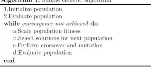
[image:4.595.58.303.462.572.2]2.1 Simple Genetic Algorithm
Fig. 1. Simple Genetic algorithm
GA is optimization search techniques useful in a number of practi-cal problems. The robustness of Genetic Algorithm is method with it’s behaviour to find the global optimum in a hypothesis. GA’s ran-dom, directed is search for locating the globally optimal solution. Randomized and directed GA is specially for finding the globally optimal solution. GA is useful as tool for a genetic representation for the feasible solution. We get a population of encoded solutions. We have a fitness function that evaluates the optimality of each so-lutions. Genetic operators generate a new population from existing
populations. The GA is iterative process of population evolution for sequenced generations. After and in between generation,each solution has fitness which gives to decide the next chromosomes to do the mating.Fitter is selected for meting and other are dis-carded from the pool. The fitter is selected by and from fitness val-ues for next generation. The selected chromosomes then has to go for crossover and mutation operation. The main and important op-eration is crossover which makes a structured and randomized ex-change of alleles with crossover possibility. Crossover can be done by Pc, crossover rate. Mutation does the flipping of the allele of a chromosome by mutation probability. The mutation plays impor-tant role to do this by restoring the lost of genetic material. Scaling is another operation which is useful for maintaining the steady se-lecting pressure in objective function.
It is an objective that GA should not converge towards the optimal solution by taking much of iterations. In this section, we discuss the role of the parameters in controlling the behavior of the GA. We also discussed the techniques proposed in the literature for op-timization of SPS problem for enhancing the performance of GA . The significance of pc and pm in controlling GA performance has long been acknowledged in GA research [7]. The crossover probability pccontrols the rate at which solutions are subjected to crossover. The higher the value of pc, the faster are the new so-lutions introduced into the population. As pc, increases, however, solutions can be disrupted faster than selection so, typical values of pc, are in the range 0.5-1.0.
Mutation is only a secondary operator to restore genetic material. Nevertheless the choice of pmplays important role in GA perfor-mance and has been emphasized in DeJongs work [25]. Large val-ues of pm, transform the GA into a solely random search algo-rithm, while some mutation is required to prevent the premature convergence of the GA to suboptimal solutions. Typically pm, is chosen in the range 0.005-0.05. We must thanks to DeJong for his the Efforts made to improve GA performance in optimization. De-Jong introduced the ideas of overlapping populations and crowd-ing in his work also. In the case of overlappcrowd-ing populations, newly generated offspring replace similar solutions of the population, pri-marily to sustain the diversity of solutions in the population and to prevent premature convergence. However,the crowding factor (CF) is introduced in this technique which has to be tuned to certain op-timal GA performance. In all the techniques described above, no emphasis is placed on the choice of pcand pm. pc, and pmis still left to the user to be determined statically prior to the execution of the GA. The idea of adaptive mutations and crossover is already employed to improve GA performance. Our approach for find-ing SPSP (software project schedule Problem) also uses not only Crossover and mutation adaptive probabilities but also adaptive fit-ness, but in a manner different from these previous approaches. In the next section, we discussed the motivation for having adaptive probabilities of crossover and mutation, and describe the methods adopted to realize them. In this paper, We used adaptive probabil-ities of crossover and mutation to see the effect of keeping simple track of diversity and taking linear load of convergence. Another advantage of our approach is to provide a solution to the problem of choosing the optimal values of the pc , and pm. (We referred crossover and mutation probability as pcand pm, respectively).
3. SOFTWARE PROJECT MANAGEMENT
3.1 Objectives
to produce profit, knowledge or something else of the organizations interest. Each software project has its own main objective which is defined at the very beginning. It is the task of the software project management process to ensure that software project main objec-tive is achieved. There are some common things that most of the projects share among themselves, e.g.:
·Specific start and threshold date.
·Time schedule,Direct cost, Indirect cost, budget and quality con-straints.
·Particular attention to get the target result.
Software Project management is the application of logical and algo-rithmic knowledge, skills, software tools and different techniques to meet the user´s requirements of the particular project. Software Project management, knowledge and practices are best described in terms of their some of s/w engineering processes eg. waterfall model, RAD, Spiral model. These processes can be placed into five process groups and nine knowledge areas. These groups are Re-quirement engineering, Design and analysis, coding, testing and integration (closing). These areas are project integration manage-ment, project scope managemanage-ment, project time managemanage-ment,project cost management, project communications management, project risk management and project procurement management, project quality management, project human resource management. There are three very important threads that we can find in almost all the software projects: Cost (Money), Schedule (time) ,and per-formance (quality). Two of them we may not exceed - Cost and Duration (Time) and the third one quality must be at least as re-quired by the customers. Above mentioned processes are actually a processes of managing a number of others, mutually dependant sub-processes each having its own objective, but contributing to the main project objective. We will see in the next section about project manager´s role and time management as this aspects are more fo-cused and related to our SPSP.
3.1.1 software Project Manager. A Software PM is a person who is responsible for the project. He/she may lead the software development towards a successful or, sometimes unsuccessful soft-ware product. A Softsoft-ware PM must have a set of competencies that make him/her appropriate person for such a duty. A project man-ager, besides leading the project, should have well communications with other related instances involved in and around the project other than software related technical problems. He has to play a role of interface that the best software PM must play. He must keep com-mon and important relations intact with project sponsors and users. Software PM is directly responsible to the project sponsor as the sponsor is the one who orders a project to be executed. Project sponsor usually defines some specific boundaries (e.g. budget, time, quality) and monitors them closely. That’s why AGA approach is not only useful for the Software PM but for the quality oriented project as our approach considers some of the aspects of SEE. Users are those who usually specify the requirements and negotiate technical details of realization that are of high importance to them. When we talk about software development, a common situation is that the client orders some extensions of already existing systems, or wants some new systems that are compatible to other existing systems. In any case, very usual things are change requests dur-ing development or after finishdur-ing the original project. That’s why we defined some flexible software engineering oriented constraints that has to be met during the scheduling of project.
3.1.2 Software project Time Management (SPTM). SPTM is a subset of project management that includes the processes required to ensure timely completion of the project. It consists of problem
definition, TPG ( Tasks precedence graph), event and activity se-quencing, schedule (DUR) estimating, schedule development ac-cording to target schedule, and schedule control. Since, time is one of the most important management factor and parameter that must be obeyed during software project development (and in SDLC), it will involve a lot of planning and reviewing on monthly, weekly or even daily basis. We come across the term Milestone in SPTM. De-fined and target Milestones shows Umbrella activities with WBS (work breakdown structure ) points in the SPM. Milestones are generally associated with important baselines and results. They are defined using time and appropriate deliverables. In another words milestones define end of certain project development phase.
4. SOFTWARE COST ESTIMATION (SCE)
There are main seven steps that is generally adapted in SCE as per the SEE [4].
Step 1. Establish objectives.
Step 2. Plan for required data and resources. Step 3. Write down software requirements. Step 4. Work out in detail work (WBS) as we can. Step 5. Use different independent techniques and sources. Step 6. Compare and Iterate budgeted estimates.
Step 7. Followup.
Out of these seven step, we work out only on roughly on step 1 and 2 and Step 5. We tried to define the problem, requirements in terms of hard and soft constraints and schedule the project with one technique i.e. by AGA.
4.1 Effort, COCOMO Models
There are various COnstructive COst MOdels developed by Barry W. Boehm and others. Estimating effort of software is product of productivity and size of team. The unit of effort is man-month (MM) or person-month (PM) which is calculated in terms of KDSI (thousands of delivered source instructions) by following equa-tion [4].
MM= 2.4 (KDSI)1.05.
Also, the development schedule (TDEV) in months is given as TDEV= 2.5 (MM)0.38
The above equation is a basic model applicable to the large majority of software projects [4]. According to COCOMO model a man-month (MM) is equal to 152 hours of working time.
Table no.2 shows Effort and Duration for three different types of project as per the COCOMO model. We assumed the calculated efforts (by COCOMO Model) as one of the inputs to our project. Further calculation, evaluation and comparison with our model is done by following equations.
T DEV = 3×(M M)0.328
(1)
HC= 0.666×(M M)0.672
(2) Above equations are also used for calculating the constrain factor, the effort and head count.
5. PROBLEM DEFINITION AND FORMULATION [?]
Table 2. Notations ,symbols and meanings. Notations Meaning
MM man-months
PM Person-Months
KDSI Thousands of delivered source instructions
TDEV Development time
HC Head Count
GSCH Schedule derived by our approach using GA CDTi COCOMO Calculated duration CODTi COCOMO Optimistic duration
= 0.86×CD AGODTi Optimistic duration
obtained by our AGA approach CPDTi COCOMO pessimistic duration
of task Ti=1.6×CD EFavg Stretch out effort of the project EFpa The Pessimistic effort at analysis phase EFpd The pessimistic effort at design phase EFpi The pessimistic effort
at implementation phase
EFp The pessimistic effort of whole project. TPHC Total project head count.
EMF Effort multiplier factors
Pc Crossover rate
Pm Mutation rate
sth Schedule number in generation χ(AGSHDs) Modified Fitness of sthSchedule FCs≡F(AGSHDs) Fitness of sthSchedule Ps Total Penalty of sthschedule NDs Normalised duration of sthschedule SEmax Maximum salary of employee
among all employees TCHCs Total COCOMO head count
of sthschedule
AGSHDs Schedule obtained by our genetic approach of sthschedule
CPSHDs COCOMO pessimistic of sthschedule COSHDs COCOMO optimistic of sthschedule DPs Degree of penalty of sthschedule Pavg Average penalty of generation Pmax Maximum penalty of generation Pmin Minimum penalty of generation NHCPs, Normalised head count Penalty NTPs, Normalised total time Penalty NITPT i Normalised task incompleteness penalty TNITPs Total Normalised Incompleteness
[image:6.595.334.542.68.392.2]Task Penalty of sthschedule
Table 3. Formulae for Effort and Duration according to the types of
project.
Organic MM = 2.4 (KDSI)1.05
TDEV= 2.5 (MM)0.38
Semidetached MM= 3.3 (KDSI)1.12 TDEV=2.5 (MM)0.35 Embedded MM=3.6(KDSI)1.20
TDEV= 2.5(MM)0.32
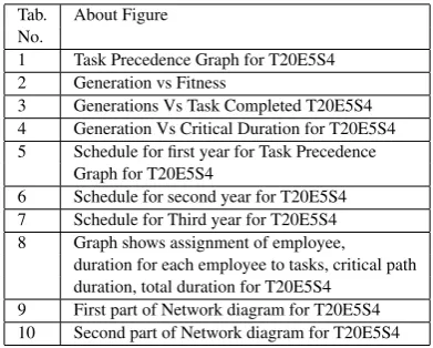
Table 4. Tables and their description. Fig. Figure´s Description
No.
1 Athours and suggested Pm 2 Notations ,symbols and meanings 3 Formulae for Effort and Duration according
to the types of project 4 Tables and their description 5 Figures and their description 6 A Sample example of solution
in terms of Schedule representation
7 Input:Configuration file [9] showing mathematical notations for T10E5S4 as an example
8 Input:Task Properties for T20E5S4 9 Input:Employee Properties for T20E5S4 10 Output:Employee working times for T20E5S4 11 COCOMO and AGA durations for T20E5S4 Where,
CODTi≤AGADTi≤CPDTi 12 Output:Tasks duration in Months with
employee for T20E5S4
13 Output:Xover Vs Avg Computation time for T20E5S4
14 Comparative chart of our and Ting-Tang approach for G2 Group 15 Comparative chart of our and
Ting-Tang approach for G3 Group. 16 Comparative chart of our
[image:6.595.334.541.71.356.2]and Ting-Tang approach for G4 group.
Table 5. Figures and their descriptionT20E5S4 means 20 Tasks, 5 Employees, 10 Skills example
but employees possesses 4-5 skills.
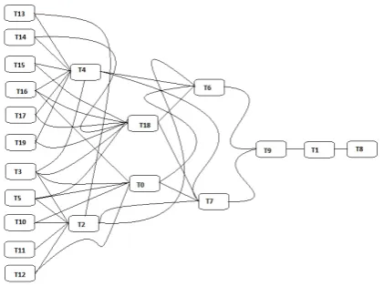
Tab. About Figure No.
1 Task Precedence Graph for T20E5S4 2 Generation vs Fitness
3 Generations Vs Task Completed T20E5S4 4 Generation Vs Critical Duration for T20E5S4 5 Schedule for first year for Task Precedence
Graph for T20E5S4
6 Schedule for second year for T20E5S4 7 Schedule for Third year for T20E5S4 8 Graph shows assignment of employee,
duration for each employee to tasks, critical path duration, total duration for T20E5S4
9 First part of Network diagram for T20E5S4 10 Second part of Network diagram for T20E5S4
• Let T be a set of tasks, T={Ti, i=0,....,n-1} where n is the number of tasks,
• Let E be a set of employees, E={Ei, i=0,....,e-1} where e is number employees,
•Let S be a set of skills, S={Si, i=0,...,m-1}, where m is the total number of skills.
•Let ES be a set of skill of employees,
ES={ESi,i=0,....,m-1}where m is the number of skills and
•EF be the effort required for the tasks in T,
EF={EFTi, i=0,...,n-1}where EFTi is the effort required for task Ti.
[image:6.595.64.284.78.600.2] [image:6.595.339.535.397.554.2]task skill matrix i.e TS,
where TS={TSij, i=0,....,n-1, j=0,...,m-1}
Each elements TSijof task skill matrix S is either 0 or 1, depending on whether task Ti requires skill Sj as
T Sij =
1 if T ask Tirequires skill Sj.
0 Otherwise.
The dependence [39] between the tasks is given by task depen-dency matrix (TD) of size of n×n. Its elements are given as,
T Dik=
1 if T ask Tidepends upon task Tk.
0 Otherwise.
[image:7.595.71.282.330.487.2]Finally, AGSHD is a n×e sized task assignment matrix of dura-tion (in months) assigned to each employee on various tasks. The duration may be in years, months, quarters or weeks. TD matrix is obtained from task precedence graph (TPG). The Task Prece-dence Graph shows the precePrece-dence relation between the tasks, is an acyclic Graph, G(T,EG) where The T represents the set of all task nodes included in the project and EG is the set of edges between de-pendent tasks [?]. A sample TPG for 10 tasks, 5 employees and 10 skills is shown in Fig 1. There are various types of tasks in a project
Fig. 2. Task Precedence Graph for T20E5S4
[55]. These are Start to Start (SS), Start to End (SE), End to Start (ES), and End to End (EE). In this paper, we have considered the tasks of SE type. Once a task starts for such tasks, it has to end without fail but by maintaining parallel or concurrent mechanism. Each task has associated with the optimistic as well as pessimistic values of effort and head count. Here, we have made the average of the pessimistic values of 3 SPM phases.
EFpa= 2×EF (3)
EFpd= 1.5×EF (4)
EFpi= 1.25×EF (5)
Epavg= 1.583333∗EF (6) Where, EFavgis stretch out effort of the project ( project maximum effort),
?EFpais the Pessimistic effort at analysis phase,
?EFpdis the pessimistic effort at design phase,
?EFpiis the pessimistic effort at implementation phase and
?EFpis the pessimistic effort of whole project.We calculated all the above corresponding duration CPD,COD using equation1 We have taken average effort as threshold value and hard constraint in our problem. We have 25% managerial margin to work for schedul-ing software project apart from CMM (Capability Maturity Model) model under consideration. CMM’s one of the principles says that 30 PC FSP should be kept as extra staff for substitution in case of critical situation. This paper gives scheduling of software project by considering some hard and soft constraints which is described in next subsection.
We used an indirect constraints handling i.e. objectives optimiza-tion by satisfying the constraints. In general, penalties are given for violated constraints. Some GAs allocate penalties for wrongly in-stantiated variables also for the distance up to a feasible solution. The generality of penalty gives reduction of the problem to simple optimization. The described and defined constraints for our SPSP (Software Project Scheduling Problem) are given and listed bellow. 5.0.1 Hard constraints. The tasks in given SPS problem are to be assigned to employees subject to the following hard constraints [5]. (1) All skills must be matched. The employee must have skills
re-quired for the tasks to be done.
(2) Task precedence graph must be satisfied during an assignment of a task to an employee.
5.0.2 Soft constraints. Also the following soft constraint are considered to obtain a better schedule.
(1) At least 80 PC of task’s head count should be as per values cal-culated by COCOMO-II.2000 and may differ at most±1 for each task head count. This is managerial adjustment, normally given by industry to the PM, to add or remove one employee to maintain the quality of the project. But, This adjustment is directly related to effort.
(2) Cost of the project should be below the average cost calculated by COCOMO-II.2000 calculation.
(3) Employee may not be overloaded more than 50% of his/her capacity.
OLE i≤0.5×CE i (7) OL and C are the overload and capacity respectively. Capacity of employee is how much employee can do quality work in one unit time. (The capacity is described in section IIIA). (4) Work should be equally distributed amongst employees as far
as possible.
(5) Equal importance should be given to project cost and duration. (6) For maintaining the quality, each duration of task should be
nearer to the optimistic duration (COD).
(7) The total number of employees for project tenure should be in between 80% and 100% of Head count calculated by COCOMO-II.
120%of TPHC >=
n
X
i=1
TPHC is total project head count.
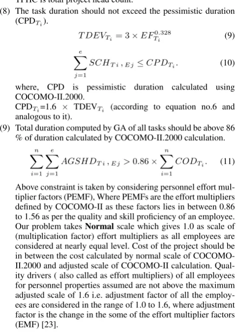
(8) The task duration should not exceed the pessimistic duration (CPDTi).
T DEVTi= 3×EF
0.328
Ti (9)
e X
j=1
SCHT i,E j≤CP DTi. (10)
where, CPD is pessimistic duration calculated using COCOMO-II.2000.
CPDTi=1.6 × TDEVTi (according to equation no.6 and analogous to it).
(9) Total duration computed by GA of all tasks should be above 86 % of duration calculated by COCOMO-II.2000 calculation.
n X
i=1
e X
j=1
AGSHDT i,E j>0.86× n X
i=1
CODTi. (11)
Above constraint is taken by considering personnel effort mul-tiplier factors (PEMF), Where PEMFs are the effort mulmul-tipliers defined by COCOMO-II as these factors lies in between 0.86 to 1.56 as per the quality and skill proficiency of an employee. Our problem takesNormalscale which gives 1.0 as scale of (multiplication factor) effort multipliers as all employees are considered at nearly equal level. Cost of the project should be in between the cost calculated by normal scale of COCOMO-II.2000 and adjusted scale of COCOMO-II calculation. Qual-ity drivers ( also called as effort multipliers) of all employees for personnel properties assumed are not above the maximum adjusted scale of 1.6 i.e. adjustment factor of all the employ-ees are considered in the range of 1.0 to 1.6, where adjustment factor is the change in the some of the effort multiplier factors (EMF) [23].
6. PROPOSED AGA APPROACH
6.1 Motivations
A software project scheduling is CSP(Constrained Satisfying prob-lem) with objective optimisation. We require pushing energy to meet optimal solution after getting the optimal space. Not only this, but also, we need another property of finding new space of solu-tion in optimal search. Interestingly, The trade-off between these properties is hiddenly packaged in values of pcand pmand also in crossover type. Usually, in practice,we take large values of pc (0.5-1.0) and small values of pm(0.001-0.05), In our approach, we put this trade-off by varying pc, and pmadaptively in response to the fitness values of chromosomes. pc, and pmare increased when the population is about to get stuck at a local optimum and are de-creased when the population in solution space is scattered. To vary pc, and pm, adaptively, for preventing premature conver-gence of the GA to local optimum. We should able to identify whether the GA is on right optimum path of convergence. For detecting the convergence ,we have to see average fitness value
fof the population in relation to the maximum fitness value fmax of the population. The minimum the value of fmax-f, more is the convergence to an optimum solution, it means a population scat-tered in the solution space.pcand pm has to be increased if GA converges to local optimum when fmax-fdecreases. Pc, and pm has to be increased if solutions come towards scattered pool.
pm α fmax−f (12)
pc α fmax−f (13)
We use the difference in the average and maximum fitness values, fmax -f, as a benchmark for detecting the convergence.†f is
also denoted by fava in adaptive mutation, crossover in next
section.It has to be observed in the above expressions that pcand pmdo not depend on the fitness value of any particular solution, and have the same values for all the solutions of the population. Consequently, solutions with high fitness values as well as solutions with low fitness values are subjected to the same levels of mutation and crossover. When a population converges to a globally optimal solution (or even a locally optimal solution), pc, and pm, increase and may cause the disruption of the near-optimal solutions. The population may never converge to the global optimum.
[image:8.595.54.296.71.408.2]To overcome the above-stated problem, we need to preserve good solutions of the population. This can be achieved by having lower values of pcand pmfor high fitness solutions and higher values of pcand pmfor low fitness solutions. This can be seen and realised in the B.4 and B.6 subsections of VII. the high fitness solutions aid in the convergence of the GA, the low fitness solutions prevent the GA from getting stuck at a local optimum. The value of pm, should depend not only on fmax- f, but also on the fitness value f of the solution. Similarly, pcshould depend on the fitness values of both the parent solutions. The closer f is to fmax, the smaller pm, should be, i.e.,pm, should vary directly as fmax- f. Similarly, pc, should vary directly as fmax- f, where f is the larger of the fitness values of the solutions to be crossed.
Fig. 3. Adaptive Genetic algorithm
6.2 Steps in AGA
6.2.1 Step 1. Initiation.. Initiation consists in creating an ini-tial population specified number of individuals chromosomes. The writers use individual representation in the form of gene strings containing information about methods and values of processes pri-ority. The initial population is created randomly. Particular genes assume values chosen randomly with equal probability from their variability interval. Activity priorities, allocated randomly in the initial population, are modified in consecutive steps of the algo-rithm until a solution that corresponds to the shortest duration of the project is obtained. Therefore, the AGA enables the user to find optimal values of priorities that determine the sequence of allocat-ing tasks to employees, to activities. The algorithm is thus a tool that may help PM in their everyday work of making decisions and setting priorities.
6.2.2 Step 2. Individuals assessment.. This procedure is used to calculate project duration, and thus it enables chromosomes fea-sible solutions assessment. To assess the solutions generated by AGA, the authors worked out the heuristic algorithm for tasks to employee allocation and calculating the shortest project duration presented in the next section.
6.2.3 Step 3. Protection of the best individual.. The individual chromosome from the initial population for which the objective function value is the best the shortest project duration is remem-bered. The best individual protection also-called exclusive strategy is a special additional reproductive procedure. The best adapted in-dividual, among all from former generations, does not always pass to a new population. Exclusive strategy is used as the protective step against the loss of that individual.
6.2.4 Step 4. Calculating value of individuals adaptive fitness function.. AGAs are used to look for the best adapted individu-als for which the fitness function value is the highest. The study focuses on finding the solutions of minimization problems. In this case, it is necessary to convert the minimized objective tion into maximized fitness function. The calibrating fitness func-tion prevents premature convergence of the evolufunc-tionary algorithm, which would result in finding a local optimum and not a global one.
6.2.5 Step 5. Checking the termination condition.. The action of the algorithm can be stopped in two cases: after performing a speci-fied number of iterations when the number of the current generation is greater than the maximum value assumed, and when, after some number of iterations, there are no better solutions than in previous generations. If the termination condition is not met, a selection of individuals is carried out as the next step.
6.2.6 Step 6. Selection procedure (Elitism).. Chromosomes se-lection consists in choosing individuals that will take part in pro-ducing offspring for the next generation. Chromosomes having the highest fitness function value are the most likely to produce new individuals. The last step is repeated for each individual in the pop-ulation.
6.2.7 Step 7. Crossover (Adaptive) . The task of crossover is to recombine chromosomes by exchanging strings of genes between parents chromosomes. The different crossovers are employed in the study. Strings of genes in the parents chromosomes ahead of the point of crossing are not changed, only genes behind that point are exchanged between parents.
6.2.8 Step 8. Mutation (Adaptive). Mutation involves random change of one or more genes of the selected chromosome, with probability equal to mutation frequency. Calculation of the fitness
function value for each individual in a new generation, the best in-dividual protection, selection procedures, crossover, and mutation are repeated cyclically until the termination condition of the algo-rithm is met. Then the result of algoalgo-rithms action, i.e., the solution to the problemthe way of using skilled employee, the project du-ration, and beginning and finishing of each task is given. The best solution corresponds to the individual having the lowest value of the assessment function the shortest or minimal project duration.
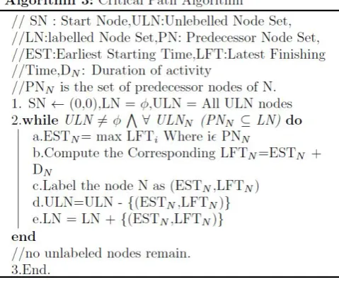
6.3 The Critical Path Procedure
[image:9.595.321.561.244.443.2]Following is the CPP is used in our approach to find and compare them with previous individual’s CPT to get optimum duration AGAD.
Fig. 4. Critical Path Algorithm
The assignment of tasks to employees are given on the devotion basis. We have choice to do the division of devotion in percentage. The gene value of chromosome is an integer in the range 0 to 8. That is, we have set of devotions in gene values with percentage considered as per following equation. If employee Eiis assigned tasks Tj , and gene value is ”1” then his or her devotion is 12.5 % of his(r) capacity . The capacity is property of Full time Soft-ware Professional (FSP) and its unit may be hours/day, days/week, hours/week. e.g. an employee can give 10 hours ”means” :if em-ployee works with capacity of 40 hours/week and his devotion is 25%. The devotion of employee can be given as
Devotion= g
Gmax
×100 (14)
6.4 Solution Representation in our approach
We proceed to describe the elements of a solution for the problem. A solution can be represented with a matrix AGSHD =(xij) of size
[image:10.595.129.294.340.473.2]ExT, where xijε[0,1]. The value xij represents the fraction of the working time that the employee Eidedicates to the task Tjin terms of months. A sample example of a problem solution is given in Table II, where a software project with 7 tasks is performed by a team of 5 employees. ’1’ indicates 100%.
Table 6. a Sample example of solution in terms of Schedule representation.
t0 t1 t2 t3 t5 t6
e0 0.125 0.625 1.0 0.375 0.125 0.625
e1 0.625 0.25 0.625 0.125 1.0 0.125
e2 0.375 1.0 0.125 1.0 0.625 0.625
e3 1 0.625 0.375 0.375 0.375 0.375
7. OPERATIONS, MATHEMATICAL MODELING AND ADAPTIVE FITNESS [?]
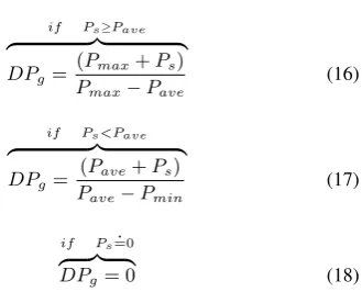
7.1 Modified objective function
Modified objective function is defined as
χ(SHDs) =F(SHDs)×(1 +DPg) (15)
if Ps≥Pave
z }| {
DPg=
(Pmax+Ps)
Pmax−Pave
(16)
if Ps<Pave
z }| {
DPg =
(Pave+Ps)
Pave−Pmin
(17)
if Ps=0.
z }| {
DPg = 0 (18)
In this way, the penalty function is kept free from any pre-defined or user defined constants, and the degree of penalty can vary ac-cording to the level of violation instead of being constant during the schedule process. The outlines of the adaptive mutation and crossover operators used in the current work, based on the meth-ods suggested by Srivinas and Patnaik (1994) but modified and described in next subsection. Pmand Pc represent a number that demonstrate the task duration shifted by mutation in the individ-ual and exchanged by crossover between the pairs. In the follow-ing formulations, the probability of mutation and cross-over depend on the fitness value of the solutions, and vary according to the fit-ness value. Therefore, the user is free from defining any value for those [53].
7.2 Fitness for AGA
The calculation and flow of the fitness for our model is sequenced in following manner.sthnumber in every equation indicates
sched-ule number or chromosome number in generationFitness of chromosome for sthschedule is given by
F Cs=
1
N Ds+Ps
(19)
,where Ps= Total Penalty of sthschedule,
N Ds=SHDs/ADs (20)
where, ND is Normalised duration,AD is Average Duration for sth schedule.
7.3 Project Duration (Schedule)
An each completed task is checked according to the TPG. For each individual, the sequence and the task completion is checked and penalty is given if the task is not completed. The constant penalty and reward technique is adapted to get good individuals, instead of making it invalid,completely. The project duration is cal-culated by
AGSHDs= e X
i=1
n X
j=1
DV(Ei,Tj) (21)
where,
DV(Ei,Tj)=devotion of employee Eito T ask Tjin months. (22)
7.3.1 Project (Schedule) Cost. The total schedule cost (SC) or project cost (PC) is obtained by summation of multiplication of devotion of each employee with each task and salary of each employee per month.
SCs= e X
i=1
n X
j=1
DV(Ei,Tj)×SEEi (23)
Maximum cost of the project is calculated by,
M SCmax= n X
i=1
CP SHDs×SEmax (24)
where, SEmaxis maximum salary of employee among all employ-ees.
7.4 Total Schedule penalty
Total penalty [32] is addition of penalties regarding time,individual task and head count. There are some competing objectives which may give the delay to get the right solution. We have example of making equal distribution of employees in project which is exactly opposite to the head count constrain. Making trade off in the contra-dictory objectives is must and common in project management [5]. The solution is to make the one of them hard and other one soft or make the both constrained soft. The total schedule penalty is calcu-lated and given by
Ps=N HCPs+N T Ps+T N IT Ps (25) where, NHCPs, NTPs, TNITPs are normalised head count, total time and task incompleteness penalty respectively.
the hard constraint is, HC of each task should be±1of Head count calculated by COCOMO.
HCPTi=
0 if Condition1
|CHCTi±1−AGHCTi| Otherwise
(26)
Condition1≡CHCTi±1
.
=GHCTi (27)
N HCPs= Pn
i=1HCPTi
T CHCs
(28)
where TCHCsis total COCOMO head count of sthschedule. 7.4.2 Threshold penalty (Time penalty) . The threshold penalty is calculated by taking the difference between AGSHD and CP-SHD.
T Ps=
rate∗(CP SHDs−AGSHDs) if Condition1
1×10⁹ if Condition2
(29)
Condition1≡COSHDs<=AGSHDs<=CP SHDs (30)
Condition2≡GSHDs> CP SHDs (31) Where,rate is penalty per unit time ( We kept rate= 1 penalty/months), AGSHD is schedule obtained by our genetic ap-proach, CPSHD is COCOMO pessimistic schedule and COSHD is COCOMO optimistic schedule.In SPM, schedule is also called as project duration or DUR or DU.
N T Ps=
T Ps
CP SHDs
(32)
NTPsis Normalised time penalty.
7.4.3 Penalty For Individual Incomplete Task [9]. The penalty of individual task is called incompleteness. This incompleteness is duration difference between optimistic duration and GA obtained duration of the task.
n X
i=1
N IT PTi= n X
i=1
(AGODTi−CODTi)/GP DTi. (33)
T N IT Ps= Xn
i=1N IT PT i (34) The incompleteness is normalised by above equation.
7.5 Adaptive Mutation
Mutation is done to change the direction search space as lowest fitness values continuation doesnt provide good solution. Mutation rate is changed according (to Togans [53] following formula) pro-vided the chromosome has worst fitness in the pool.
Pm=
0.5(fmax−f)/(fmax−fave) f≥fave.
(fave−f)/(fave−fmin) f < fave. Here,f is the fitness of an individual,fave is the average fitness value of the population,fmaxandfminare the maximum and min-imum fitness value of an individual in the population respectively. Pm is mutation rate.
We have done simply the summation of all the objective function and calculate the fitness value. Every objective is given same pref-erence. The weight is equally distributed in the objectives itself. The proposed SGA with adaptive approach for modified fitness function given by Togan, Patnaik is considered to get the more suit-able fittest chromosome from adaptive approach [53].
7.6 Adaptive Crossover
The crossover operator mimics the way in which bisexual repro-duction passes along each parents good genes to the next genera-tion [18]. Two parent create two new offsprings by combining their genes typically according to following pseudo code. Crossover uses both inheritance and variation to improve the performance of the population while retaining its diversity of population [8]. In our ap-proach, following flow of operation of crossover is experimented. Pseudocode for the same is given bellow.
7.6.1 Adaptive Elitist Crossover (EX). where:
P(t) is equal to Pc; Comments ? The selection process in SGA is always preceded by the crossover process. But ,in the EX above method, both processes are integrated. The entire population is ran-domly shuffled during the first step. Then,two new vectors are cre-ated by crossover from each successive pair of parental vectors. Two best vectors are singled out and taken as offspring to the next population. ? Some times premature convergence may be due to the reason of traditional way of elitist selection application on the level of the entire population. So, we can apply this an EX elitist selection on the family level.
Pc=
(fmax−f0)/(fmax−fave) f0≥fave.
0 f0< f
ave.
Where, f’ is the larger of the fitness value of the solutions to be crossed [53]
7.7 Selection :Elitist strategy
Elitist strategy is utilized for avoiding destroying the best individual per generation. Specifically described as follows: If the next gen-eration of groups of individual fitness value is less than the current population of individual fitness value, the best individuals in the current groups or adaptation value is greater than the value of the next generation of the best individual fitness multiple individuals directly copied to the next generation. The elitist strategy ensures that the current best individual will not be destructed by crossover and mutation operations [43]. We used separate ´adaptive crossover and elitist selection´, Elitist adaptive crossover.
7.7.1 Stopping Criterion. Though, it is, usually, expected that solution quality improves with the additional generations in GA. Typically, genetic algorithms terminate after a predetermined num-ber of generations passed or after a sequence of consecutive gener-ations without objective function improvement. Alternatively, the algorithm can terminate after the population is sufficiently homog-enized, as measured by objective function variance [54]. We are interested in the temporal (generational) performance in elitism se-lection strategy [42]. we opted to utilize a maximum generation as a stopping criterion..
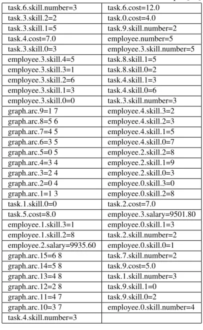
8. INPUT OUTPUT TABLES
properties and TPGs. The outputs in terms of all these properties has been given as the parameters and properties in INPUT Table-7 to 9. In tern, These parameters are taken as inputs to our imple-mentation. The table-10 onward all tables represents outputs of our approach.
Table 7. INPUT:Configuration file showing mathematical notations for T10E5S4 as an example [56]
task.6.skill.number=3 task.6.cost=12.0 task.3.skill.2=2 task.0.cost=4.0 task.3.skill.1=5 task.9.skill.number=2 task.4.cost=7.0 employee.number=5 task.3.skill.0=3 employee.3.skill.number=5 employee.3.skill.4=5 task.8.skill.1=5
employee.3.skill.3=1 task.8.skill.0=2 employee.3.skill.2=6 task.4.skill.1=3 employee.3.skill.1=3 task.4.skill.0=6 employee.3.skill.0=0 task.3.skill.number=3 graph.arc.9=1 7 employee.4.skill.3=2 graph.arc.8=5 6 employee.4.skill.2=3 graph.arc.7=4 5 employee.4.skill.1=5 graph.arc.6=3 5 employee.4.skill.0=7 graph.arc.5=0 5 employee.2.skill.2=8 graph.arc.4=3 4 employee.2.skill.1=9 graph.arc.3=2 4 employee.2.skill.0=3 graph.arc.2=0 4 employee.0.skill.3=0 graph.arc.1=1 3 employee.0.skill.2=8 task.1.skill.0=0 task.2.cost=7.0
task.5.cost=8.0 employee.3.salary=9501.80 employee.1.skill.3=1 employee.0.skill.1=3 employee.1.skill.2=8 task.2.skill.number=2 employee.2.salary=9935.60 employee.0.skill.0=1 graph.arc.15=6 8 task.7.skill.number=2 graph.arc.14=5 8 task.9.cost=5.0 graph.arc.13=4 8 task.1.skill.number=3 graph.arc.12=2 8 task.9.skill.1=0 graph.arc.11=4 7 task.9.skill.0=2
graph.arc.10=3 7 employee.0.skill.number=4 task.4.skill.number=3
Fig. 5. Generation Vs Fitness T20E5S4
Table 8. INPUT : Task Properties for T20E5S4. Task Effort CD CPD CHC Skills
ID (PM) (Mths) (Mths) Required
Task0 11 6.5 10.54 3.3 1,5,9
Task1 3 4.3 6.88 1.3 3,6,9
Task2 12 6.7 10.84 3.5 2,6
Task3 8 5.9 9.49 2.6 0,8,9
Task4 12 6.7 10.84 3.5 0,5,7
Task5 7 5.6 9.08 2.4 1,7
Task6 15 7.2 11.67 4.0 0,6,8
Task7 21 8.1 13.03 5.1 4,5
Task8 11 6.5 10.54 3.3 1,3
Task9 18 7.7 12.39 4.6 5,7,9 Task10 10 6.3 10.22 3.1 1,3,5
Task11 8 5.9 9.49 2.6 0,1,2
Task12 17 7.5 12.16 4.4 6,7,8 Task13 15 7.2 11.67 4.0 0,5,9 Task14 16 7.4 11.92 4.2 0,1,7
Task15 7 5.6 9.09 2.4 3,7
Task16 10 6.3 10.22 3.1 4,6,8
Task17 10 6.3 10.22 3.1 0,1
Task18 11 6.5 10.54 3.3 0,1,5
[image:12.595.335.540.74.311.2]Task19 15 7.2 11.67 4.0 6,8
Table 9. INPUT : Employee properties for T20E5S4.
Emp Id Salary Months work load Skills factor
0 9793 3 1 0,1,5,7,9
1 9545 3 1 0,1,6,8,9
2 10131 3 1 1,2,4,8
3 10252 3 1 0,5,6,9
[image:12.595.59.296.141.655.2]4 10944 3 1 0,3,7,8
Table 10. OUTPUT:Employee working times for T20E5S4. Employee Time No. of Task
Per Employee
0 25.875 15
1 22.025 15
2 27.975 14
3 24.4 15
4 21.525 16
9. RESULT AND DISCUSSION
9.1 Analysis and Discussion
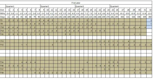
[image:12.595.72.276.148.479.2]Fig. 8. Schedule for first year for Task Precedence Graph for T20E5S4
Fig. 9. Schedule for second year for T20E5S4
rate and mutation rate. At the same time, the search property has been balanced by restricting crossover and mutation. To insure the best chromosome pass to the next generation, we immediately
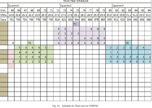
Fig. 10. Schedule for Third year for T20E5S4
Fig. 6. Generations Vs Task Completed T20E5S4
This can get away from local optimal and avoid premature conver-gence. Also the convergence speed increases [19]
We have taken approach elitist selection. Though the AGA plays indirect role of elitist approach. We, also, took various penalties and reward to the parameters of the objective functions
.Experienc-Fig. 7. Generation Vs Critical Duration for T20E5S4
[image:14.595.54.563.446.611.2]Fig. 11. Graph shows assignment of employee, duration for each employee to tasks, critical path duration, total duration for T20E5S4
Fig. 12. First part of Network diagram for T20E5S4
COCOMO-II effort estimation, schedule calculation, Head count for our paper and implementation. In preliminary run, we used the right extinctive selection for 2 to 5 individuals (having less fitness) for having zero production rate for some generation to discard the some but little number of chromosomes which dont tends to give super-individuals. We used elitist selection scheme which enforces to go through selection along with their parent by making some individual duplicates by constrained wise changes in the chromo-somes.Comparison Table of simple GA(Ting [56]),AGA by our ap-proach and ACO (Ting [56]) shows that AGA has good result than others. Figure 2 and onwards gives the various graphs and chart. These graphs gives the behaviour of AGA with parallelism. In par-allelism ,if some skilled employees is idle then we allocate that task to the employee by making allocation of randomized genes.
The execution of sequenced task are considered as per the princi-ples of parallelism of project management.We see if all tasks are completed first within group of sequenced parallel tasks, in turn, we can start the next sequence of task immediately after the com-pletion of all the tasks in the previous sequence. All predecessors of that task must be completed before going to execute successor tasks or follower tasks. Equal distribution of the work employee is considered for the sake of making equilibrium in the division of a task but it is exactly opposite to the head count of the task required.
9.2 Computational AGA results
[image:15.595.53.555.316.519.2]Fig. 13. Second part of Network diagram for T20E5S4
Table 11. COCOMO and AGA durations for T20E5S4 Where, CODTi≤AGADTi
≤CPDTi.
CD COD AGAD CPD
Task0 6.59 5.66 6.00 10.54 Task1 4.30 3.70 6.38 6.88 Task2 6.78 5.83 6.38 10.84 Task3 5.93 5.10 4.88 9.49 Task4 6.78 5.83 5.63 10.84 Task5 5.68 4.88 7.50 9.09 Task6 7.29 6.27 6.75 11.67 Task7 8.14 7.00 8.63 13.03 Task8 6.59 5.66 7.50 10.54 Task9 7.74 6.66 6.38 12.39 Task10 6.38 5.49 7.13 10.22 Task11 5.93 5.10 5.63 9.49 Task12 7.60 6.53 6.38 12.16 Task13 7.29 6.27 7.88 11.67 Task14 7.45 6.41 6.38 11.92 Task15 5.68 4.88 5.25 9.09 Task16 6.38 5.49 5.25 10.22 Task17 6.38 5.49 9.75 10.22 Task18 6.59 5.66 5.63 10.54 Task19 7.29 6.27 6.00 11.67
one generation to another generation. The fitness value takes a con-stant path after some generation as it increases, it takes concon-stant value. Though, the fitness gives constant value but it gives some different solutions by considering all the composite components of the schedule. We studied combination of different crossover types with adaptive Pc,Pm. The generation is set to 500 for this specific
Table 12. OUTPUT: Tasks duration in Months with employee for T20E5S4.
Emp0 1 2 3 4 AGAD
Task0 2.25 1.875 1.875 0 0 6
Task1 1.125 1.5 0 3 0.75 6.375
Task2 0 1.5 2.25 2.625 0 6.375
Task3 0.375 1.875 0.375 1.125 1.125 4.875
Task4 0 1.875 0 0.75 3 5.625
Task5 3 1.125 1.875 0 1.5 7.5
Task6 1.125 1.875 1.875 0.75 1.125 6.75
Task7 3 0 3 2.625 0 8.625
Task8 0.75 1.875 2.625 0 2.25 7.5 Task9 0.75 2.25 0 1.5 1.875 6.375
Task10 0 3 0.75 2.625 0.75 7.125
Task11 2.25 1.5 1.125 0.375 0.375 5.625 Task12 1.125 0 2.625 1.875 0.75 6.375
Task13 2.25 2.625 0 3 0 7.875
Task14 1.125 0 0 3 2.25 6.375
Task15 2.25 0 0 0 3 5.25
Task16 0 1.125 1.5 2.25 0.375 5.25 Task17 2.25 1.5 1.875 3 1.125 9.75
Task18 2.25 0 2.625 0 0.75 5.625
Task19 0 1.875 3 0.75 0.375 6
problem of 20 Tasks, 5 Employees, 10 Skills. We got the following as outputs
[image:16.595.98.252.383.615.2]Table 13. Xover Vs Avg Computatin time for T20E5S4.
Xover Avg (SGA) Avg (AGA) Methodology Computation Computation
One point 250 90
Two pont 210 75
Uniform 290 100
Selective 360 120
—addition of each gene to get the value of time required for tasks, employees working time
—getting the distribution of employee over the number of tasks —team size for completing the each task
—concurrent parallel adjustment of each employee with the task assigned to skilled employee
—time required to complete the project i.e. schedule —Cost of the schedule
—fitness of the schedule.
The figures 2 to 10 shows the above things in the chart. The cost and time decreases as we do progress from one generation to an-other generation. The fitness value takes a constant path after some generation as it increases, it takes constant values. Though the fit-ness gives constant value but it gives some different solutions by considering all the composite components of the schedule. We put crossover rate 0.9, mutation rate 0.01 initially and then the effect of adaptive approach is observed which makes Pmand Pmchanges according to the fitness from generation to generation as stopping criteria is 500 number of generations as different type of crossover requires different computation time.
9.3 Gantt Chart of sample example as an representation of task, breakdown
The schedule created is shown in Gantt Chart which shows tasks assigned to skilled employees, critical path, dependency between tasks as per input TPG, Starting and ending days and duration of each tasks. It shows the sequence and flow of the tasks with starting and ending point with employee allocations in slots. Fig.6 shows the graph which shows same information as above for schedule of 20 Tasks, 5 employees, 10 skills example. It shows the concept of SS, SE, ES, EE examples also and can be used for showing it.
9.4 Comparative discussion
Here, we compared the results of our model’s with Ting,Tang’s [56] results. Somewhere, it has been found that the result of ACO ( Ant colony optimization ) are better and some time our results are. This observation can also be seen in the results of Ting,Tang. ACO is better than GA for some of the smaller problems and our approach GA put behind the ACO and the result of Ting and Tang. Our results are good when problem becomes complicated and complex due to GA’s global optimization nature, due to combination of crossover types and changes in the mutation rate according to fitness of individual. Our results produced may give hope of making project manager feel satisfy about the schedule.
10. CONCLUSION
Not only SGA or GA but also AGA gives various chance to us to take tour of various parameters variability to get the optimistic
solution. All operators like adaptive crossover, adaptive mutation, adaptive fitness gives different combinations of the solution. It is the god gifted mechanism that gives chance of using constant as well as mathematical modelled penalties to get the best optimal solution. The constant penalty approach gives some what less result than adaptive approach in the penalty.
[image:17.595.356.517.329.528.2]In preliminary run, we set the pool of chromosome in such a way that, after preliminary run the chromosomes in the pool get some combinations of the super individual, best individual, normal indi-viduals and zero product individual so that the natural test of GA is kept on. In preliminary run, we got some good solution in chromo-some pool to propagate to the next generation. Figure 3 to 7 gives different graphs .These graphs gives the behaviour of AGA with parallelism in scheduling [30]. In parallelism ,if some skilled em-ployees is idle then we allocate that task to the employee by making allocation of randomized genes. The execution of sequenced tasks are considered as per the principles of parallelism of project man-agement [15] .We see, if all tasks are completed first within group of sequenced parallel tasks, in turn, we can start the next sequence of task immediately after the completion of all the tasks in the pre-vious sequence. All predecessors of that task must be completed before going to execute successor tasks or follower tasks. Equal dis-tribution of the work employee is considered for the sake of making equilibrium in the division of a task but it is exactly opposite to the head count of the task required .
Table 14. OUTPUT:Comparative chart of our and Ting-Tang approach for G2 Group
Employee possesses 4-5 skills.
Group Instance Algorithm Duration G2 5e10t ACS-SPSP 22.94651 GA 23.63111 AGA 20.875 10e10t ACS-SPSP 14.21091
GA 16.28071 AGA 16.125 15e10t ACS-SPSP 8.032931
GA 8.2231
AGA 8.125
20e10t ACS-SPSP 6.306531 GA 6.01912
AGA 6.00
Table 15. OUTPUT:Comparative chart of our and Ting-Tang approach for G3 Group.Employee possesses 6-7 skills
Group Instance Algorithm Duration G3 5e10t ACS-SPSP 22.11891 GA 23.15251 AGA 23.625 10e10t ACS-SPSP 14.20831
GA 13.2522 AGA 11.625 15e10t ACS-SPSP 8.2368 GA 8.05221
AGA 7.75
20e10t ACS-SPSP 6.020961 GA 6.284971
[image:17.595.357.518.471.673.2]