Bayesian Inference on a Cox Process Associated with a Dirichlet Process

Bayesian Inference on a Cox Process Associated with a

Dirichlet Process

Larissa Valmy

LAMIA (EA4540) Universit´e des Antilles-Guyane

BP 250 - 97157 Pointe-`a-Pitre

Jean Vaillant

LAMIA ( EA4540) Universit´e des Antilles-Guyane

BP 250 - 97157 Pointe-`a-Pitre

ABSTRACT

In ecology and epidemiology, spatio-temporal distributions of events can be described by Cox processes. Situations for which there exists a hidden process which contributes to random ef-fects on the intensity of the observed Cox process are consid-ered. The observed process is a generalized shot noise Cox pro-cess and the hidden propro-cess is a Poisson propro-cess associated with a Dirichlet process. The distributional properties of quadrat counts are presented and bayesian inference is proposed for estimating and predicting parameters of interest in the model. Illustrations are given from weed spatial count data and disease mortality data.

General Terms:

Point process, Bayesian statistics, Mixture models

Keywords:

point process, Cox process, bayesian inference, ecology, epidemi-ology

1. INTRODUCTION

In ecology and epidemiology, distributions of events like disease occurrences, predator arrivals or plant locations can be considered as realizations of a point process, of which each point represents a single event. The point process theory has been presented and discussed in [2], [3] and [8]. Statistical procedures for analysing point process realizations can be found in books ([6]; [22]; [12]; [19]) and a lot of papers deal with applications in special situa-tions (e.g. [7]; [11]; [4]; [25]). Some studies are based on counts of events in sampling units ([5]), and some others on event spatial positions or occurrence dates ([25]), and also distance sampling ([16]). Perry et al. ([20]) discussed appropriate selection and use of method for analyzing spatial point patterns in plant ecology. One may refer to [19] for papers about statistical tools for spatial point processes. [5] discussed recently about spatial point process models for forest inventories exhibiting overdispersion. In applications in which overdispersion is assumed, Cox process modeling is a com-mon choice since this class of point processes is wide enough to take into consideration many features. Thus, [26] presented various scientific fields in which the Cox process, also known as doubly stochastic Poisson process, occurs. The intensity processλ(.)of

such a process on a measured space(X,B, ν) is a random field related to its driving random measureΛ(.)as follows :

Λ(B) =

Z

B

λ(x)ν(dx), (1)

for any elementBofB. In expression (1),Λ(B)is a random vari-able which stands for the expected number of points inB. Thus, modeling a Cox process is equivalent to modeling either its inten-sity or its driving measure ([24]). For example, [4] described a spe-cific class of Cox processes, namely shot-noise G Cox processes, by modelingΛ(.)with a shot-noise G-measure.

2. DISTRIBUTIONAL PROPERTIES OF COUNT MIXTURES

LetNbe a Cox process with intensity processλon spaceX de-fined by :

∀x∈X, λ(x) = M

X

j=1

ajK(x, yj) (2)

whereKis a kernel function such thatK(., y)is a probability den-sity function onX for anyyinXandM is the random number of contributions. Theyjare a realization of a point processLon

Xwith positive real marksajidentically distributed according to a probability lawGon R+, and independent of theyj. IfL is a homogeneous Poisson process with scalar intensityµ and theai are equal to the same value, thenλis a standard shot noise process ([17]), and thenNis a standard shot noise Cox process. Moreover, if the bandwidth ofKis a random variable, thenNis a generalized shot noise Cox process ([18]). In expression (2),ajis the contribu-tion of eventyjto the intensityλ.

In this paper, the contributionsajare assumed to follow a Dirichlet processG([13],[9]) with base measureG0and concentration

pa-rameterαdenoted byDP(α, G0). Therefore, there is no

indepen-dence condition on theajas in many models but a weaker condition of exchangeability provided by De Finetti’s theorem, see for exam-ple [10]. In fact the contributionsajare conditionally independent givenG. This provides a way of taking into account correlation be-tween marks and mixed environmental effects. Theyjare assumed to be occurrence locations of a homogeneous Poisson process with parameterµdenoted byHP P(µ). In other words,

(aj)|G i.i.d∼ G

(yj) ∼ HP P(µ)

G ∼ DP(α, G0).

(3)

The following propositions give some distributional properties of the counting measure associated withNwith respect to concentra-tion parameterα.

PROPOSITION 1. Let N be a Cox process on the measured space(X,B, ν)with intensiy defined by equations (2) and (3), then

∀A∈ B, E(N(B)) =µE(a1) Z

X

Z

B

K(x, y)ν(dx)ν(dy)

and

V(N(B)) =E(N(B))

1− 1

α+ 1E(N(B))

+µE(a21) Z

X

Z

B

K(x, y)ν(dx)

2

ν(dy).

PROOF. Taking into account (1) and (2), then for any element BofB,

Λ(B) = M

X

j=1

aj

Z

B

K(x, yj)ν(dx). (4)

Since theyj are uniformly distributed onX conditionally toM, the expectation ofΛ(B)conditional onMis

M E(a1) Z

X 1

ν(X)

Z

B

K(x, y)ν(dx)ν(dy)

and the final result for E(N(B)) is obtained from E(M) =

µν(X).

Similarly, the second moment ofΛ(B)conditional onMis

M E(a2 1)

Z

X 1

ν(X)

Z

B

K(x, y)ν(dx)

2

ν(dy)

+M(M−1)E(a1a2) Z

X 1

ν(X)

Z

B

K(x, y)ν(dx)ν(dy)

2

.

E(a1a2) = (E(a1))2α/(α+ 1); E(M(M−1)) = (µν(X)) 2

and V(N(B)) =V(Λ(B)) +E(Λ(B)) lead us to the final result.

PROPOSITION 2. With the same conditions as in proposition 1, let(B1, B2)be an element ofB2withB1∩B2=∅. The covariance betweenN(B1)andN(B2)is

Cov(N(B1), N(B2)) =

µE(a21) Z

X

Z

B1

K(z, y)ν(dz)

Z

B2

K(x, y)ν(dx)

ν(dy)

− 1

α+ 1E(N(B1))E(N(B2)).

PROOF. Since N is a Cox process, then Cov(N(B1), N(B2)) =Cov(Λ(B1),Λ(B2)).

On the other hand,

E(Λ(B1)Λ(B2)) =

E

M

X

j=1

aj

Z

B1

K(x, yj)ν(dx) M

X

k=1

ak

Z

B2

K(x, yk)ν(dx)

!

=E

M E(a2 1)E

Z

B1

K(x, y1)ν(dx) Z

B2

K(x, y1)ν(dx)

+E

M(M−1)E(a1a2)E Z

B1

K(x, y1)ν(dx) Z

B2

K(x, y2)ν(dx)

The final result is obtained from

E(M) =µν(X), E(a1a2) = (E(a1))2α/(α+ 1) and

E(M(M−1)) = (µν(X))2.

Let us consider count data inrdisjoint subsets ofX. WhenG0

be-longs to a probability distribution family parameterized bybandK a kernel family parameterized byσ, we have the following result :

PROPOSITION 3. Let N be a Cox process on the mea-sured space (X,B, ν) with intensiy defined by equations (2) and (3) and let B1,· · ·, Br ber disjoint elements of B. Con-sider G0 parameterized by b and K parameterized by σ. Un-der independent priors for α, b, µ and σ, the posterior distri-bution of(α, b, µ, σ,(aj)j=1,...,M, M), conditional on counts in

B1,· · ·, Br, is proportional to :

p(α)p(b)p(σ)p(µ)p(a1, . . . , aM|α, b, M)

(µν(X))M

M! e

−µν(X)

×

r

Y

i=1

Λ(Bi)N(Bi)e

with the conditional joint distribution of theajobtained from the following expression :

aj|a1, . . . , aj−1∼

α

α+j−1G0+ 1

α+j−1 j−1 X

k=1

δak. (6)

TheΛ(Bi)depend on(σ,(aj)j=1,...,M, M)as described in (4). PROOF. Conditionally to processλ, theN(Bi)are independent counts following respectively a Poisson distribution with parameter Λ(Bi). The associated conditional likelihood is then multiplied by the joint prior distribution of the parametersα, b, µ, σ, a1, . . . , aM andM. The Bayes theorem is then applied.

Equation (5) is obtained from the predictive law representation pre-sented by [1].

In the sequel,Kis assumed to be an isotropic gaussian kernel with bandwidthσ. Another aspect of the model is the limits when the spatial influence parameterσtends to zero or when the concentra-tion parameterαtends to zero or infinity.

PROPOSITION 4. With the same conditions as in proposition 1, considerB and B0

two disjoint elements of Band letK be an isotropic gaussian kernel with bandwidthσ. Then

1) lim

σ→0E(N(B)) =µE(a1)ν(B), 2) lim

σ→0

V(N(B))

E(N(B)) = 1−

µE(a1)

α+ 1 ν(B) +

E(a2 1)

E(a1) , 3) lim

σ→0Cov(N(B), N(B

0

)) =µ2_(E(a 1))2

α

α+ 1ν(B)ν(B

0

),

4) The variance-to-mean ratio V(N(B))

E(N(B)) is an increasing func-tion with respect toα.

PROOF. 1) Λ(B) = M

X

j=1

aj

Z

B

K(x, yj)ν(dx) and for any

(x, j)∈X× {1,· · ·, M}, K(x, yj)converges toδyj({x})

asσconverges to0. This gives us

lim σ→0Λ(B) =

M

X

j=1

ajδyj(B) (7)

.

E(N(B)) = E(Λ(B)) = E M E(a1|M)E(δyj(B)|M)

. Independence of aj and yj conditional on M leads to lim

σ→0E(N(B)) =µE(a1)ν(B).

2)

Z

B

K(x, y)ν(dx) converges to 1B(y) asσ converges to 0.

Therefore

lim σ→0 Z

X

Z

B

K(x, y)ν(dx)

2

ν(dy) =ν(B)which leads us

to the final result. 3) Equation (7) leads to

E(Λ(B)Λ(B0)) = µ2_ν(B)ν(B0

)E(a1a2). On the other

hand,Cov(N(B), N(B0)) =Cov(Λ(B),Λ(B0)). Therefore, Cov(N(B), N(B0_{)) =µ}2_ν(B)ν(B0_)Cov(a

1, a2).

b

↓

α G0 µ

↓ . ↓

G P P H

& . & (aj) (yj)

& .

λθ← σ

[image:3.595.379.495.67.188.2]

↓ (N(Bi))

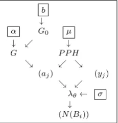
Fig. 1. Acyclic directed graph of the hierarchical model defined by (3)

withG0=Gamma(1, b)

4) From proposition 1, it results that

V(N(B))

E(N(B))=1− 1

α+ 1E(N(B))

+E(a 2 1)

E(a1) Z

X

Z

B

K(x, y)ν(dx)

2

ν(dy)

Z

X

Z

B

K(x, y)ν(dx)ν(dy)

.

Moreover, in the above equation, the third term of the right member andE(N(B))do not depend onα. Consequently, the variance-to-mean ratio is increasing withα.

Proposition 4 shows that even if the spatial influence of hidden events is negligeable (σclose to zero), count correlation may be high according to the value taken by parameterα. It is worth point-ing out that whenαequals zero, theajare all equal to each other whereas whenαconverges to infinity, theajare independent iden-tically distributed according toG0. Thus property4in proposition 4

indicates thatαis a dispersion parameter. The lowerαis, the higher the correlation betweenajis and the lower the overdispersion is.

In the sequel, the Gamma distribution with scale parameteraand shape parameterbis denoted byGamma(a, b).

3. ESTIMATION PROCEDURE

Posterior inference methods can be performed on spatial models ([14]) by implementing MCMC sampling. The model defined by expressions (2) and (3) and described by figure 1 involves two sets of unknowns, firstα, b, µ, σwhich are the parameters of interest, secondly, the positions(yj)and effects(aj)of the hidden events. Let us denote byq(.)the joint distribution of the unknowns and count data up to a constant. Then :

q((N(Bi)),(α, b, µ, σ, M,(aj, yj)j=1,···,M))∝

p(a1, . . . , aM|α, b, M)

µM

M!

p(α, b, µ, σ)

eµν(X) r

Y

i=1

Λ(Bi)N(Bi)_e−Λ(Bi)

(8)

As expressed in (4), the positions(yj) intervene in the posterior distribution of(α, b, µ, σ)in the following way :

Λ(Bi) = M

X

j=1

aj

Z

Bi

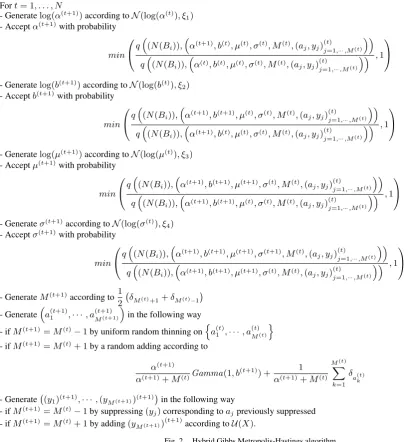
Fort= 1, . . . , N

- Generatelog(α(t+1)_{)according toN(log(α}(t)_{), ξ} 1)

- Acceptα(t+1)_{with probability}

min





q(N(Bi)),α(t+1)_{, b}(t)_{, µ}(t)_{, σ}(t)_{, M}(t)_,(a j, yj)

(t) j=1,···,M(t)

q(N(Bi)),α(t)_{, b}(t)_{, µ}(t)_{, σ}(t)_{, M}(t)_,(a j, yj)

(t) j=1,···,M(t)

,1 



- Generatelog(b(t+1)_{)according toN(log(b}(t)_{), ξ} 2)

- Acceptb(t+1)_{with probability}

min





q(N(Bi)),α(t+1)_{, b}(t+1)_{, µ}(t)_{, σ}(t)_{, M}(t)_,(a j, yj)

(t) j=1,···,M(t)

q(N(Bi)),

α(t+1)_{, b}(t)_{, µ}(t)_{, σ}(t)_{, M}(t)_,(a j, yj)

(t) j=1,···,M(t)

,1 



- Generatelog(µ(t+1)_{)according toN(log(µ}(t)_{), ξ} 3)

- Acceptµ(t+1)_{with probability}

min





q

(N(Bi)),

α(t+1)_{, b}(t+1)_{, µ}(t+1)_{, σ}(t)_{, M}(t)_,(a j, yj)

(t) j=1,···,M(t)

q(N(Bi)),α(t+1)_{, b}(t+1)_{, µ}(t)_{, σ}(t)_{, M}(t)_,(a j, yj)

(t) j=1,···,M(t)

,1 



- Generateσ(t+1)_{according toN(log(σ}(t)_{), ξ} 4)

- Acceptσ(t+1)_{with probability}

min





q(N(Bi)),α(t+1)_{, b}(t+1)_{, µ}(t+1)_{, σ}(t+1)_{, M}(t)_,(a j, yj)

(t) j=1,···,M(t)

q(N(Bi)),α(t+1)_{, b}(t+1)_{, µ}(t+1)_{, σ}(t)_{, M}(t)_,(a j, yj)

(t) j=1,···,M(t)

,1 



- GenerateM(t+1)_{according to}1

2 δM(t)₊₁+δ_M(t)−1

- Generatea(₁t+1),· · ·, a(t+1)

M(t+1)

in the following way

- ifM(t+1)_=M(t)_{−1by uniform random thinning on}n_a(t) 1 ,· · ·, a

(t) M(t)

o

- ifM(t+1)_=M(t)_{+ 1by a random adding according to}

α(t+1)

α(t+1)_+M(t)Gamma(1, b

(t+1)_{) +} 1

α(t+1)_+M(t) M(t)

X

k=1

δ

a(_kt)

- Generate (y1)(t+1),· · ·,(yM(t+1))(t+1)

in the following way - ifM(t+1)_=M(t)_{−1by suppressing(y}

j)corresponding toajpreviously suppressed - ifM(t+1)_=M(t)_{+ 1by adding(y}

[image:4.595.54.469.65.508.2]

M(t+1))(t+1)according toU(X).

Fig. 2. Hybrid Gibbs Metropolis-Hastings algorithm

Expression (8) enables convenient use of the MCMC algorithm proposed in figure 2.

It is worth noticing that independent priors were chosen forα, b, µ andσ. Consequently, the Metropolis-Hastings ratios at the different steps of the algorithm may be simple to calculate, particularly for updating parametersα,bandµ.

For each individual parameter, the MCMC sampling enables in-ferences made via posterior marginal distribution. In fact, at the completion of the MCMC run, we have a posterior joint distribu-tion sample for the parameters of interest which provides a good approximation of their posterior probability law.

[23] offered a set of suggestions for choosing among models by ex-amining the posterior distribution of the log-likelihood under each model. They introduced the deviance information criterion in aim-ing to combine measure of fit and complexity (effective number of parameters). The resulting criterion is the difference between the

posterior mean of the deviance and the deviance at the posterior mean which can be easily calculated from the MCMC posterior sample.

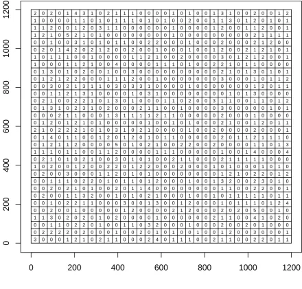
4. ANALYSIS OFIBICELLA LUTEACOUNT DATA

Data provided by [16] are considered. They consist of742weeds (Ibicella lutea) in an australian farming paddock of area1200×

1200 square meter. This weed dispersal mechanism is through seeds falling to the ground from ripen fruits. Additionally, fruits are carried away from plants by mammals. These latter unobserved events can be mathematically considered as the realization of an hidden process.

Table 1. Dispersion and spatial autocorrelation test results forIbicella luteawith respect to grid size

grid Mean Variance Dispersion Dispersion Moran Moran

size index pvalue index pvalue

×10−5 _×10−1 _×10−2

42 46.25 142.33 3.08 5 3.32 3.9 82 _{11.56 18.60 1.61 157 1.74 4.16}

162 2.89 3.98 1.38 6 1.50 0.075 322 _{0.72 0.87 1.20 1 0.64 0.37}

Table 2. Bayesian inference results forIbicella luteacount data

Mean Median Standard error 95%HPD

α 22.516 21.974 6.367 (11.920,36.761)

b 5.157 5.880 1.750 (2.150,7.456)

µ 20.139 19.145 6.598 (9.808,34.285)

σ 0.048 0.033 0.024 (0.030,0.097)

different grid sizes and the dispersion and Moran autocorrelation indices were calculated and tested for each grid size (table 1). A significant overdispersion was found for each of the spatial scales which were considered. The spatial autocorrelation was signifi-cantly positive for grid sizes2k_×2k_{, k ≥ 2(table 1). This led} us to apply the Cox process model defined from expressions (2) and (3). Thenµstands for the expected number of dispersal events whereasσis a seed dispersal parameter : the closerσis to zero, the shorter are the dispersal distances. We assume that the contribu-tionsajto weed intensity follow a Dirichlet process centered on a Gamma distribution with scale parameter equal to unity and shape parameterb, denoted byGamma(1, b). In fact the Gamma distri-bution is frequently used in environmental effect modeling ([24]). Here parameterbis the expected contribution to intensity for a dis-persal event sinceGamma(1, b)is the marginal distribution of any ai. When concentration parameterαtends to zero, the contribu-tionsaj are strongly and positively correlated. Whenαtends to infinity, these contributions are independent.

The bayesian inference results are summarized in table 2 using pos-terior means, medians, standard deviations and95%highest poste-rior density (HPD) intervals. The bayesian mean number of hidden events is around20. Posterior mean contribution is5.16. The in-fluence parameter bayesian mean is0.048. The concentration pa-rameter estimates are around22. The Bayesian deviance calculated at the posterior mean was choosen as criterion of goodness-of-fit ([23]). In table 5, the bayesian deviance result indicates that the hy-pothesis of equality of some contributions is more likely than the one of independent contributions.

In addition to information on structure of weed communities in crops such as the one provided by [21], these results may give some relevant information about unobserved events in the framework of weed control management. The proposed approach provides esti-mates of hidden process parameters influencing the weed dispersal and can be integrated into weed management programs.

5. ANALYSIS OF CHRONIC LOWER

RESPIRATORY DISEASES DEATH NUMBERS

[image:5.595.325.547.85.302.2]

A set of data from Georgia (USA) was analyzed. These data avail-able at the Web site http://www.georgiastats.uga.edu/ consist of counts of death cases in each of the159counties of Georgia, for chronic lower respiratory diseases (CLRD) in2007. For these dis-eases, death occurrences are sometimes the consequence of unob-served events due to environmental factor effects which generate

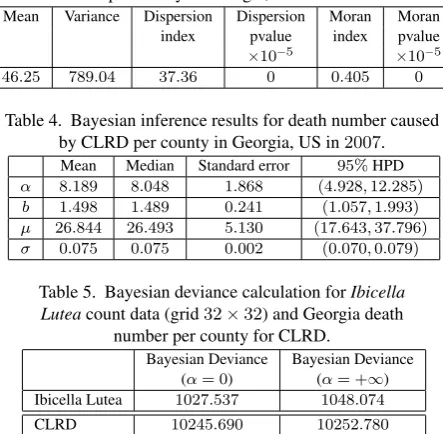
Table 3. Dispersion and spatial autocorrelation test results for death number per county in Georgia, US in2007for CLRD. Mean Variance Dispersion Dispersion Moran Moran

index pvalue index pvalue

×10−5 _×10−5

46.25 789.04 37.36 0 0.405 0

Table 4. Bayesian inference results for death number caused by CLRD per county in Georgia, US in2007. Mean Median Standard error 95%HPD

α 8.189 8.048 1.868 (4.928,12.285)

b 1.498 1.489 0.241 (1.057,1.993)

µ 26.844 26.493 5.130 (17.643,37.796)

σ 0.075 0.075 0.002 (0.070,0.079)

Table 5. Bayesian deviance calculation forIbicella Luteacount data (grid32×32) and Georgia death

number per county for CLRD.

Bayesian Deviance Bayesian Deviance (α= 0) (α= +∞) Ibicella Lutea 1027.537 1048.074

CLRD 10245.690 10252.780

clustering. However, it is possible to formulate a bayesian cluster model taking into account such unobserved process of cluster cen-ters ([15]).

Figure 4 shows the case counts for each county for CLRD along with the neighbourhood links between counties. The neighbour-hood weight is based on whether or not two counties share border-lines with each other. The dispersion index and the Moran spatial index based on this neighbourhood were calculated (table 3). The corresponding p-values indicate a very strong overdispersion and positive spatial autocorrelation for CLRD.

Tables 4 and 5 show the results of bayesian inference for these dis-eases. The bayesian mean number of hidden events is26.84for chronic lower respiratory disease. The bayesian deviance is weaker under the hypothesis of equal contributions compared the one un-der the hypothesis of independent contributions. In other words, the equality of contributions is more likely than their independence.

6. CONCLUSION

In this article, a model of Cox process associated with a Dirichlet process was proposed with an emphasis on modeling spatial distri-butions of events generated by hidden occurrences. Event contri-butions are distributed according to a Dirichlet process centered on a Gamma distribution. A hybrid Gibbs-Metropolis-Hastings algo-rithm was developed. It provides the posterior distribution for the following parameters : expected number of hidden events per spa-tial unit, expected contribution per hidden event, spaspa-tial influence of hidden events and dispersion index due to hidden events. The hypotheses of contribution equality and contribution independence are compared by means of bayesian deviance calculation. Applica-tion to real data shows the potential of the method considered.

7. REFERENCES

[1] D. Blackwell and J.B. Macqueen. Ferguson distributions via polya urn schemes.Annals of Statistics, 1(2):353–355, 1973. [2] P. Bremaud. Point Processes and Queues: Martingale

[image:6.595.83.524.124.545.2]

0

200

400

600

800

1000

1200

0

200

400

600

800

1000

1200

3 0 0 1 0 0 0 0 0 0 1 0 1 0 0 2 0 0 0 0 0 0 0 0 1 1 0 0 1 1 1 2 0 2 0 1 0 0 2 0 0 2 0 2 1 1 1 1 1 0 1 2 0 0 1 1 0 0 2 0 2 1 0 0 0 2 1 3 2 1 0 2 1 0 2 1 1 2 4 0 2 0 3 1 1 3 2 3 0 1 0 1 1 2 0 2 0 2 1 0 0 0 0 0 1 0 0 0 0 1 0 2 0 2 1 0 1 0 1 0 0 1 1 0 0 0 0 0 1 2 0 2 0 2 1 2 1 3 0 1 1 1 1 2 1 1 0 0 2 2 2 1 1 1 4 0 5 0 0 1 2 0 2 0 1 2 1 1 0 0 1 0 1 2 1 2 2 1 2 2 1 1 2 0 1 0 2 3 2 1 1 4 1 2 2 2 0 1 3 0 2 0 2 2 0 0 0 1 1 0 3 2 3 3 0 2 2 0 0 1 1 2 1 3 0 0 0 0 0 1 2 1 2 0 0 1 0 0 0 0 0 0 1 1 1 1 0 0 1 1 2 0 0 0 0 1 2 0 1 1 0 0 0 0 0 1 0 0 1 0 1 1 1 0 0 0 0 1 0 0 0 0 1 1 1 3 1 0 1 0 0 0 0 0 0 0 1 1 2 0 1 0 2 0 0 1 2 1 0 0 1 1 0 0 2 0 0 1 0 2 1 1 0 2 0 0 1 2 0 2 2 3 2 5 0 3 0 3 0 3 0 3 1 0 4 0 0 1 0 1 1 1 0 0 1 0 1 3 0 0 1 0 0 0 0 0 1 1 0 1 0 0 0 0 1 0 0 0 0 1 0 0 1 1 0 0 1 0 2 0 1 1 1 1 1 1 0 1 2 0 0 1 0 1 1 3 2 3 0 1 2 0 0 0 1 1 0 2 0 0 0 0 0 1 0 0 2 0 0 0 0 2 0 1 2 0 0 3 0 0 0 1 0 0 0 0 0 0 2 0 3 0 0 1 2 4 1 1 2 1 0 2 1 1 1 1 1 0 3 1 0 0 0 2 0 2 0 0 1 0 4 1 2 1 0 3 1 0 2 0 0 0 1 1 0 0 0 2 1 0 1 0 1 0 1 1 1 2 0 0 0 0 0 0 0 0 0 0 0 0 0 0 0 0 1 0 1 0 0 1 0 1 0 0 0 0 1 0 0 0 0 0 1 0 1 1 0 0 2 0 0 0 0 0 0 2 1 0 1 0 1 1 0 1 0 0 0 0 1 0 0 0 1 1 0 1 1 0 0 0 1 1 0 0 0 0 2 1 0 2 0 0 0 0 1 0 0 0 0 0 0 2 0 0 0 0 0 0 1 0 1 0 2 2 1 0 1 0 0 1 0 2 0 1 1 0 0 2 0 1 0 0 1 0 1 1 0 0 2 1 0 1 0 0 0 0 0 0 0 0 0 0 0 0 0 0 0 0 0 0 0 0 0 0 0 0 0 0 0 0 0 0 0 0 0 0 0 0 0 0 0 0 0 0 0 0 0 0 0 0 0 0 0 0 0 0 0 0 0 0 0 0 0 0 2 0 0 2 0 0 1 0 1 0 1 0 0 2 0 2 0 0 0 3 0 0 0 0 2 0 1 0 0 1 1 1 1 1 2 1 2 1 0 1 3 1 0 2 1 0 2 0 2 2 3 1 0 0 3 2 2 3 2 2 0 2 1 3 1 2 0 1 0 0 1 1 2 2 1 1 0 0 0 0 1 0 0 1 1 0 0 1 1 0 0 0 0 0 3 1 0 0 0 0 2 1 1 0 0 1 0 1 0 0 1 0 0 0 0 0 0 0 0 0 0 1 0 0 0 0 0 0 0 0 2 0 0 1 1 0 0 0 0 1 1 0 1 0 0 0 0 0 1 0 0 1 1 2 2 0 0 1 1 0 2 3 0 4 5 1 1 2 2 2 0 1 4 1 2 2 1 1 0 1 3 1 1 3 1 1 1 2 2 1 2 2 2 0 1 1 0 0 1 2 3 2 1 1 0 1 1 0 2 0 0 1 0 2 0 0 0 2 2 1 1 2 0 0 0 0 0 0 0 1 0 0 0 0 0 0 0 0 1 0 0 0 1 0 0 0 1 1 0 0 1 2 1 0 1 0 1 0 0 2 1 2 1 0 1 1 1 0 0 1 1 0 1 0 0 1 0 1 1 0 0 0 0 0 1 0 0 1 1 1 0 0 0 4 1 1 0 2 0 0 4 3 0 1 1 0 1 2 0 1 2 1 0 1 1 0 1 1 1 2

Fig. 3. 32×32regular grid ofIbicella luteaspatial count data

[3] P. Bremaud.Point Processes and Their Statistical Inference. 1991.

[4] A. Brix and J. Chadœuf. Spatio-temporal modeling of weeds and shotnoise cox processes.Biometrical Journal, 44:83–99, 2002.

[5] Comas C., Mateu J., and Delicado P. On tree intensity estima-tion for forest inventories: Some statistical issues.Biometrical Journal, 23(6):994–1010, 2011.

[6] A.D. Cliff and K. Ord.Spatial Processes: Models & Applica-tions. 1981.

[7] J. Cuzick and R. Edwards. Spatial clustering for inhomoge-neous populations. Journal of the Royal Statistical Society: Series B, 52:73–104, 1990.

[image:7.595.153.461.63.402.2]

Fig. 4. Neighbourhood link and death number per county for Georgia state, US in2007for CLRD.

[9] P. Diaconis and D. Freedman. Prior distributions on spaces of probability measures.The Annals of Statistics, 2:615–629, 1974.

[10] P. Diaconis and D. Freedman. De finetti’s theorem for markov chains.The Annals of Probability, 8(1):115–130, 1980. [11] P. Diggle, B. Rowlingson, and T. Su. Point process

method-ology for on-line spatio-temporal disease surveillance. Envi-ronmetrics, 16:423–434, 2005.

[12] P.J. Diggle. Statistical Analysis of Spatial Point Patterns. 1983.

[13] T.S. Ferguson. A bayesian analysis of some nonparametric problems.The Annals of Statistics, 1:209–230, 1973. [14] A. Kottas, J. A. Duan, and A. E. Gelfand. Modeling disease

incidence data with spatial and spatio-temporal dirichlet pro-cess mixtures.Biometrical Journal, 49:1–14, 2007.

[15] A.B. Lawson.Bayesian disease mapping: hierarchical mod-eling in spatial epidemiology. 2009.

[16] G.J. Melville and A.H. Welsh. Line transect sampling in small regions.Biometrics, 4(5):1130–1137, 2001.

[17] J. Møller. Shot noise cox processes. Advanced in Applied Probability, 35:614–640, 2003.

[18] J. Møller and G.L. Torrisi. Generalised shot noise cox pro-cesses.Advances in Applied Probability, 37:48–74, 2005.

[19] J. Møller and R. Waagepetersen. Modern statistics for spatial point processes.Scandinavian Journal of Statistics, 34:643– 684, 2007.

[20] G.L.W Perry, B.P. Miller, and N.J. Enright. A comparison of methods for the statistical analysis of spatial point patterns in plant ecology.Plant Ecology, 187(1):59–82, 2006.

[21] S.L Poggio, E.H. Satorre, and E.B. de la Fuente. Structure of weed communities occuring in pea and wheat crops in the rolling pampa (argentina).Agriculture, Ecosystems and Envi-ronment, 103:225–235, 2004.

[22] B.D. Ripley.Spatial Statistics. 1981.

[23] S.D. Spiegelhalter, N.G. Best, B.P. Carlin, and A. van der Linde. Bayesian measures of model complexity and fit. Jour-nal of the Royal Statistical Society, Series B, 4:583–639, 2002.

[24] J. Vaillant. Negative binomal distributions of individuals and spatio-temporal cox processes.Scandinavian Journal of Statistics, 18:235–248, 1991.