Thermodynamic Equilibrium of the Saturated Fluid with a Free Surface Area and the Internal Energy as a Function of the Phase Specific Volumes and Vapor Pressure

http://dx.doi.org/10.4236/eng.2015.79053

Thermodynamic Equilibrium of the

Saturated Fluid with a Free Surface Area

and the Internal Energy as a Function of the

Phase-Specific Volumes and Vapor Pressure

Albrecht Elsner

Am Mühlbach 14, D-85748, Garching, Germany Email: [email protected]

Received 17 July 2015; accepted 21 September 2015; published 25 September 2015

Copyright © 2015 by author and Scientific Research Publishing Inc.

This work is licensed under the Creative Commons Attribution International License (CC BY).

http://creativecommons.org/licenses/by/4.0/

Abstract

This study is concerned with describing the thermodynamic equilibrium of the saturated fluid with and without a free surface area A. Discussion of the role of A as system variable of the interface phase and an estimate of the ratio of the respective free energies of systems with and without A show that the system variables

(

V M S U, , ,

)

given by Gibbs suffice to describe the volumetric properties of the fluid. The well-known Gibbsian expressions for the internal energies of the two-phase fluid, namely d

(

µ T

) (

d 1T

)

−v_v⋅d

(

p T

) (

d 1T

)

for the vapor and

(

) (

)

(

) (

)

d µ T d 1T − ⋅v_l d p T d 1T for the condensate (liquid or solid), only differ with respect to the phase-specific volumes vv and vl. The saturation temperature T, vapor presssure p, and

chemical potential µ are intensive parameters, each of which has the same value everywhere within the fluid, and hence are phase-independent quantities. If one succeeds in representing µ as a function of vv and vl, then the internal energies can also be described by expressions that

only differ from one another with respect to their dependence on vv and vl. Here it is shown that

(

T

) (

p T

)

d µ d can be uniquely expressed by the volume function

(

vv+ −vl

(

vv−vl

) (

ln v vv l

)

)

. Therefore, the internal energies can be represented explicitly as functions of the vapor pressure and volumes of the saturated vapor and condensate and are absolutely determined. The hitherto existing problem of applied thermodynamics, calculating the internal energy from the measurable quantities T, p, vv, and vl, is thus solved. The same method applies to the calculation of the

Keywords

Fluid with Free Surface Area, Solution of Gibbs’s Internal Energy Equations, Chemical Potential Expression, Calculation of Entropy and Heat Capacity

1. Introduction

We are concerned here with electrically and magnetically neutral single-component matter under steady-state equilibrium conditions which are thermodynamically defined in the immediate vicinity of the critical point and below it. Between the critical gas temperature T_c and the triple-point temperature T_t (if it exists) the gas mass

M is structureless and homogeneously distributed in the vessel volume V. It is assumed that M has the critical density 1v_c =M V =1v. Below the critical point, M is decomposed as condensed mass M_l with the density

1 1

l l l

M V = v > v in the sub-volume V_l and as vapor mass M_v with the density M V_{v v} =1v_v<1v in the sub-volume V_v. This gas mass in thermodynamic equilibrium existing in two phases is called a saturated fluid. As thermodynamic theory teaches, the only independent variable of the saturated fluid that can be chosen is the saturation temperature T, since the other field variables possible, viz. vapor pressure p and chemical potential

µ, are unique functions of T.

The critical point, from the experimental perspective, is the first occurrence or vanishing of a free surface A

observed in V, which separates the volumes V_l and V_v from one another. By variation of T and M or V and observing the occurrence of A, one can define and measure the critical values v, T_c, and p_c.

The work in Section 2 is concerned with describing the thermodynamic equilibrium of the real gas. The stationary equilibrium of M in V is known from Gibbs to be expressed by the fundamental equation

(

, ,

)

V =V M S U which reproduces the functional relation among V, M, and the properties of the fluid, viz. entropy S, internal energy U, and free energy F =U−ST.

Section 3 firstly treats the equilibrium of the two-phase fluid without an internal free surface, i.e. A=0. The distributions of the masses M_l and M_v in V_l and V_v are given as functions of T. Then the equilibrium in the case A>0 is discussed where there is a third fluid phase, called the interface phase. To it is assigned the free interface energy F_i, which is identified with − ⋅A γ (γ surface tension), so that the ratio F F_i can be numerically estimated. Estimation and discussion of the role of A as system variable show that the system variables

(

V M S U, , ,

)

given by Gibbs suffice to describe the volumetric properties of the fluid with and with- out a free surface area.

In Section 4, it is reminded that the entropy and energy functions S, S_l, and S_v and also U, U_l, and U_v

assigned to the masses M, M_l, and M_v are absolute temperature functions with thermodynamic zeros. This result, which can be deduced from internal energy functions being subject to Nernst’s theorem at absolute zero, is noteworthy, because the said quantities have been treated in Applied Thermodynamic Theory for more than a century as temperature functions with arbitrarily specified constants.

Finally, in Section 5, the central task of this work, viz. finding an explicit thermodynamic expression for

(

) (

)

d µ T d p T in

[

0,T_c

]

, is tackled and then solved in Section 6. The energy functions u, u_v, u_l, sT,

v

s T , s T_l and µ, and the heat capacities c, c_v, and c_l can then be calculated from the measurable quantities v T_v

( )

, v T_l

( )

, and p T

( )

.

By means of the expression given for the volume function d

(

µ T

) (

d p T

)

many thermodynamic relations are verified in the Appendix, this in turn being evidence for the correctness of the volume function used.

2. Description of the Thermodynamic Equilibrium of the Real Gas

Thermodynamics uses intensive and extensive quantities to describe the equilibrium state of the gas mass M

enclosed in the volume V. An intensive property of the gas is the same everywhere in the volume and is therefore independent of the mass. Intensive equilibrium state quantities are the temperature T, pressure p, and chemical potential µ. They are defined by the first partial derivatives of extensive quantities [1], e.g., the internal energy U, which according to the fundamental equation is a function of entropy S, volume V, and mass

(

, ,

)

,

U =U S V M =TS−pV+µM

, , ,

, , .

V M M S S V

U U U

T p

S V µ M

∂ ∂ ∂

     

=_{ } = −_{ } =_{ }

∂ ∂ ∂

      (1)

Variations in the extensive quantities S, V, and M lead to variations in the intensive quantities T, p, and µ [2]

as follows:

, , ,

, , ,

, , ,

d d d d ,

d d d d ,

d d d d .

V M M S S V

V M M S S V

V M M S S V

T T T

T S V M

S V M

p p p

p S V M

S V M

S V M

S V M

µ µ µ

µ ∂ ∂ ∂       =_{ } +_{ } +_{ } ∂ ∂ ∂       ∂ ∂ ∂       =_{ } +_{ } +_{ } ∂ ∂ ∂       ∂ ∂ ∂       =_{ } +_{ } +_{ } ∂ ∂ ∂       (2)

By means of Maxwell’s relations [2]

(

)

(

)

, ,

M S V M

T V p S

∂ ∂ = − ∂ ∂ ,

(

)

(

)

, ,

S V V M

T M µ S

∂ ∂ = ∂ ∂ ,

(

∂ ∂p S

)

_{V M,} = − ∂ ∂

(

T V

)

_{M S,} ,

(

)

(

)

, ,

S V M S

p M µ V

∂ ∂ = − ∂ ∂ ,

(

)

(

)

, ,

V M S V

S T M

µ

∂ ∂ = ∂ ∂ , and

(

∂ ∂µ V

)

_{M S,} = − ∂ ∂

(

p M

)

_{S V,} the differentials (2) can be written in the form

, , ,

, , ,

, , ,

d d d d ,

d d d d ,

d d d d .

V M V M V M

M S M S M S

S V S V S V

T p

T S V M

S S S

T p

p S V M

V V V

T p

S V M

M M M

µ µ µ µ ∂ ∂ ∂       = +_{ } −_{ } +_{ } ∂ ∂ ∂       ∂ ∂ ∂       = −_{ } +_{ } −_{ } ∂ ∂ ∂       ∂ ∂ ∂       = +_{ } −_{ } +_{ } ∂ ∂ ∂       (3)

For the single-component gas the well-known Gibbs-Duhem relation between the intensive quantities in dif- ferential form reads [2]:

d d d 0.

S T−V p+M µ= (4)

Explicit writing gives

, , ,

, , ,

, , ,

0 d d d

d d d

d d d .

V M V M V M

M S M S M S

S V S V S V

T p

S S V M

S S S

T p

V S V M

V V V

T p

M S V M

M M M

µ µ µ ∂  ∂  ∂   = _{ } −_{ } +_{  } ∂ ∂ ∂           ∂  ∂  ∂   + __{∂ } −__{∂ } +_∂ _      ∂   ∂  ∂   + __{∂ } −__{∂ } +_∂ _      (5)

Variations in S, V, and M can be performed independently of each other. For dV = 0 and dM = 0 one thus has

(

)

,

(

)

,

(

)

,

0=S ∂ ∂T S _{V M}+V ∂ ∂T V _{M S}+M ∂ ∂T M _{S V} or

(

)

M S,

(

)

V M,

(

)

S V,

(

)

V M,

S= − ∂ ∂V T V ∂ ∂T S −M ∂ ∂T M ∂ ∂T S . Applying the identity

(

) (

) (

)

1

X Z Y

Z Y Y X X Z

∂ ∂ ∂ ∂ ∂ ∂ = − , the entropy relation can be written as

(

)

(

)

, ,

T M T V

S=V ∂ ∂S V +M ∂ ∂S M .

Using the Maxwell relations

(

)

(

)

, ,

T M V M

S V p T

∂ ∂ = ∂ ∂ and

(

)

(

)

, ,

T V V M

S M µ T

∂ ∂ = − ∂ ∂ , one arrives at the

Gibbs-Duhem form of the entropy:

, ,

.

V M V M

p

S V M

T T µ ∂ ∂     = _{ } − _{ } ∂ ∂

With dS =0 and dM = 0 one obtains

(

)

(

)

, ,

M S M S

S =V ∂ ∂p T −M ∂ ∂µ T , whereas the conditions dS =0

and dV =0 give

(

)

(

)

, ,

S V S V

S =V ∂ ∂p T −M ∂ ∂µ T .

In the following, the properties of the real gas are investigated under the condition of constant mass M in given volume V. The entropy thus has the form (6). The internal-energy expression immediately follows from

the fundamental equation, i.e.

(

)

(

)

, ,

V M V M

U =ST−Vp+Mµ=V ∂ ∂p T T−Vp−M ∂ ∂µ T T+Mµ or

(

)

( )

1 _,

(

( )

1

)

_, .

V M V M

T p T

U M V

T T

µ

∂  ∂ 

= _{ ∂} _ − _{ ∂} _

    (7)

According to relations (6) and (7), the entropy and internal energy of the gas mass are defined by the temperature derivatives of the intensive quantities µ and p and the quantities M and V. The gas volume V has the significant property that it is proportional to the gas mass M since the gas of mean density

v

−1 assumes the equilibrium-state volume V =vM. The entropy S and internal energy U are thus quantities that are proportional to M and hence absolute quantities [3]. As mentioned above, extensive and intensive quantities, both of which are given with absolute figures, are used for describing the emquilibrium properties of the gas, no matter which gas phases exist.

3. Two-Phase Equilibrium without and with a Free Surface Area

For every real gas there is a certain temperature T_c, called critical temperature, at which the gas mass M

decomposes into a low-density vapor-phase mass M_v and a high-density condensed-phase mass M_l (liquid or solid). The masses M_v and M_l are located in different subvolumes V_v and V_l, separated from one another by a free interface area A. If V M_{v v} =v_v =V M_{l l} =v_l =V M =v, the first occurrence of A in V defines the critical volume v and T_c, i.e. the critical point

(

v T, _c

)

of the gas, which for temperatures T ≤T_c is termed as a saturated fluid. Ignoring the existence of A, this fluid has the following properties:

{

}

{

}

( )

( )

( )

( )

( )

( )

( )

( ) (

) ( )

( )

( )

( )

( )

( )

(

)

( )

( )

, , ,

, , , , , , , , , 0,

, , , , , , , ,

0 0 0 for 0 ,

0 0 , , 0 ,

0 , , 0 0 .

v l v l v l

v l v l v l

l l l c v c v v c

l l c v v

l l c v v

M M M V V V X X X X S U F H G C A

X M x v s u f h g c X M x

v v T v T v v T v T v T T

s s T s v T s v T s T s

u u T u v T u v T u u T

= + = + = + = =

= = =

< < ≤ = = ≤ < < ≤

= < ≤ ≤ ≤ <

< ≤ ≤ = ≤ ≤

(8)

The relation X =xM states that the quantity X is proportional to the mass M, which means that each of the functions X (gas volume V, entropy S, internal energy U, free (Helmholtz) energy F =U−ST, enthalpy

H =U+Vp, Gibbs energy G= +F Vp, and heat capacity C=dU dT) ensures its uniqueness, has absolute value due to its thermodynamic zero, and is numerically interrelated to one another [3].

The decomposition of mass M into M_v and M_l below the critical point is intrinsicly described by [3]

, .

v l l l v v

v l l v v l l v

M xy yx M yx xy

M x y x y M x y x y

− −

= =

− − (9)

Taking x=v, x_{l v,} =v_{l v,} and y= =v v_{l v,} , Equation (9) gives 1

0 1 for 0 .

2

l v l v

c

v l v l

v v M M v v

T T

v v M M v v

− −

≤ = ≤ ≤ = ≤ ≤ ≤

− − (10)

It is seen, because of v_{v l,} =v_{v l,}

( )

T , that the mass ratios M_{v l,} M are functions of v and T.

The proof of

( )

( )

1

2

v c l c

M T M =M T M = is as follows: The positive functions y=

(

v_v−v

) (

v_v−v_l

)

and

(

l

) (

v l

)

y= v v− v −v are related by y≥y and y= −1 y. For v_v =v_l =v the functions y and y con-

verge from above and below to the same limiting value y_c. This yields y_c = −1 y_c or 1 2

c

Then equation Mv Ml =

(

v−vl

) (

vv−v

)

=1 represents the relation between the masses and specific volumes on incipient decomposition. With decreasing system temperature, more and more vapor particles con- dense into the liquid phase, i.e. the mass ratio M_v M_l becomes less than 1 and decreases with decreasing

temperature: M_v M_l =

(

v−v_l

) (

v_v−v

)

<1 and d

(

v v− l

) (

vv−v

)

 dT >0 for T<Tc.

If one investigates the temperature dependence of the volumes V_v and V_l between the critical point and absolute zero, one can generally ascertain that the volume variations are smaller than those of the masses and take opposite directions. From V V_l =

(

v M_{l l}

) ( )

vM one obtains V T_l

( )

_c V =

(

vM 2

) (

vM

)

=1 2 and

( )

0

(

( ) ( )

0 0

)

( )

( )

0

l l l l

V V = v M vM =v v, while from V V_{v l} =

(

v v_{v l}

) (

⋅ M_v M_l

)

it follows that

( ) ( )

1

v c l c

V T V T = and V_v

( ) ( )

0 V_l 0 =v v_l

( )

0 −1. Since for real gases 2.5<v v_l

( )

0 <4 the ratio V_v

( ) ( )

0 V_l 0 takes values between 1.5 and 3, with a jump occurring at the triple point. The following relations are valid:

1 1 1 1 1 1

, 1.

1 1 2 1 1 1

v l l v v l

l v l v l v

V v v V v v V v v

V v v V v v V v v

− − −

= ≥ ≥ = = ≥

− − − (11)

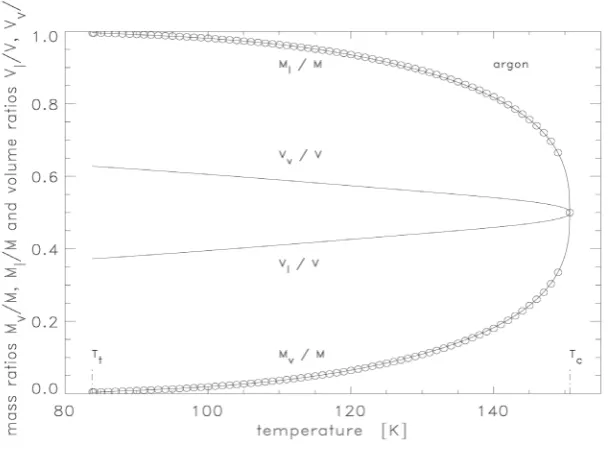
Evaluation of relations (10) and (11) is given by means of published volume data for argon in Figure 1. Let us now turn to the problem of thermodynamic treatment of the physics of the free interface surface A. As stated, the existence of A affords the possibility of distinguishing in V between two fluid phases of different

mass densities 1

v v v

M V =v− and 1

l l l

M V =v− and defining the critical point. Thermodynamic theory teaches that the intensive quantities T, p and µ have the same value everywhere in V, i.e. in the interface layer as well, in which the density decreases from 1

l

v− to 1

v

[image:5.595.163.468.460.687.2]

v− . If the length of this decrease is denoted by the distance δL, the volume δV = ⋅A δL can be assigned to the interface layer, in which the interface mass δM is located, where it holds that

(

V_lαδV

) (

+ V_v±αδV

)

=V and

(

M_l±αδM

) (

+ M_vαδM

)

=M with 0≤ ≤α 1. The fictitious quantities δV and δM , however, cannot be thermodynamically calculated, whereas both the minimum surface expansion A, resulting from intermolecular and acceleration forces, and the surface tension γ , which is a measure of the effectiveness of these forces at the surface, are measurable quantities, γ being a positive quantity [5]. The force resulting from these two yields the direction of the surface normal of A. The expansion of A depends on the shape of the vessel V. If, for example, the shape of V is chosen such that arbitrary rotation about the center of gravity of M changes the location of the interface, i.e. the height and expansion, the values of p and γ as measures of the energy density in V_{v l,} and A remain unchanged, but the distribution of

Figure 1. Mass ratio Mv M≤M Ml and volume ratio V Vv ≥V Vl of argon as

functions of the temperature. Data 3 1.8809 cm g

the interface mass δM in the newly formed volume δV is changed and this can also be reversed isother- mally and isobarically, since the free energy measures the mechanical work done. On the other hand, the redistribution of the fluid mass is a result of the changed gravitation potential in V and this can, in principle, be determined as potental energy from the height differences of A before and after rotation and hence be thermodynmically expressed by the difference in the free energy F. Thus A can be regarded as an external thermodynamic variable, and the product

(

A⋅γ

)

is measurable and constitutes a thermodynamic quantity.

Independently of prehistory, it holds for the saturated fluid that if the condition for forming a free surface between the liquid and vapor phases is given, then there is an interface particle layer, which represents a new equilibrium state described by a minimum internal energy U and simultaneously a maximum entropy S. Hence formation of the free interface surface A lowers the free energy of the fluid, F. This situation is formally taken into account by introducing the phase “interface” in keeping with the additive property of a variable X in addition to the phases “vapor” and “condensate” [6]:

{

}

(

2

)

(

)

, , , , , , , , ,

0 , 0, 0, d d 0,

0 c d , 0 c d d d .

v l v l v l i

i i i

T T

i _T i _T

M M M V V V X X X X X S U F H G C

F U S T A A T

U A T T T S A T T T

γ

γ

γ

γ

γ

= + = + = + + =

≥ = − ⋅ = − ⋅ > ≥ − ≥

≥ = − ⋅

_∫

≤ = ⋅

_∫

−

(12)

The energy term

(

− ⋅A γ

)

is interpreted as free interface energy and described by the function F_i; the newly introduced function U_i is interpreted as surface energy, and the function S_i as surface entropy. These func- tions represent reversible interface quantities of the free surface A which vanish at A=0 and also at T =T_c

because γ_c =0 and dγ dT_c =0.

Then the enlarged Gibbs relations (6) and (7) read [6]

(

)

( )

(

( )

)

2

d d d 1

d ,

d d d

d d

d ,

d 1 d 1

.

c

Tc T

T

T p

S M V A T

T T T T

T p T

U M V A T T

T T T

F U S T M V p A

µ

γ

µ

γ

µ

γ

= − ⋅ + ⋅ − ⋅

= ⋅ − ⋅ − ⋅

= − ⋅ = ⋅ − ⋅ − ⋅

∫

∫

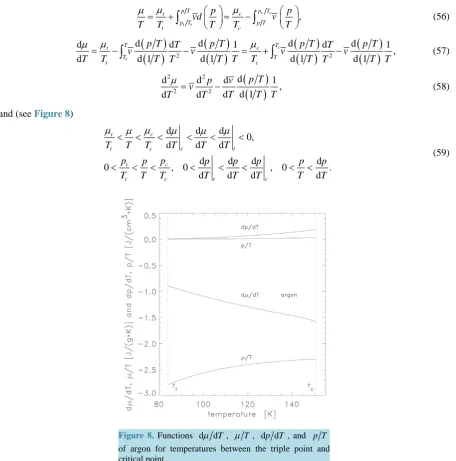
(13)

Figure 2 shows the temperature dependence of ∂ ∂ =F A F A_i , ∂U ∂ =A U_i A, and ∂ ∂ =S A S_i A for argon. In turn, these functions multiplied by A represent the area-contributions to the negative internal and free energies and positive entropy of the saturated fluid.

In order to put the interface quantity F_i in thermodynamic relation to the above-mentioned quantities δM

and δV, F_i is set equal to F

(

δM,δV

)

=µδM−p Vδ . Assuming δM =δV vˆ, δV = ⋅A δL and a mean in-

terface density 1

(

1 1

)

_{1 ˆ}

2 vv vl v

− ₊ − _{= , one obtains, because of}

i

F = −Aγ , a functional relation between surface

tension and interface quantities,

0, ˆ

p V M

p L

A v

δ µδ µ

γ = − =_ − _⋅δ ≥

  (14) which, however, remains numerically indeterminable owing to the hypothetical length δL. In turn, relation (14) allows the qualitative statement that δL is continuously increasing from 0 at T_c to values of order ₁₀−8 _cm

at T_t (see Figure 2, Figure 4 and Figure 8).

The relative energy contribution of an interface quantity to the respective system quantity depends on the ratio of the numbers of interacting particles in the interface volume δV and system volume V, i.e.

(

ˆ

) (

)

M M V v V v V V

δ = δ ≈δ , and is therefore extremely small. Despite the smallness of the order 10−8 and less [7] [10], surface effects play a great role in nature and technology. The smallness of an interface quantity shows, on the other hand, that ignoring it when studying volume properties of the fluid is completely justified. As the existence of a surface A does not change the mass M and volume V, the property of U, S, and F

being extensive quantities is maintained.

4. The Thermodynamic Zero of Thermodynamic Functions

[image:7.595.143.491.82.350.2]

Figure 2. Analysis of free-surface quantities. From fitted published surface tension data

( )

γ of argon [8] [9] and setting

( )

−γ equal to the area-specific free energy, i.e. F A_i = − <γ 0, one gets the area-specific surface energy

(

2

)

d 0

c

T

i _T

U A= −T

∫

γ T T< and the area-specific entropy

(

d d

)

d 0

Tc

i _T

S A=

∫

− γ T T T> . It holds that U_i− ⋅ =S T_i F_i= −Aγ<0. Each of these functions vanishes at T=Tc.

fluid are interrelated as follows:

(

)

( )

(

( )

)

(

( )

)

(

( )

)

d d d d

.

d 1 l l d 1 v v d 1 d 1

p T p T p T T

u v u v u v

T T T T

µ

+ = + = + = (15)

Since 0 <vl≤ ≤v vv and −d

(

p T

) ( )

d 1T =dp dT T⋅ − >p 0 for T ≤Tc, one has ul < <u uv and

(

uv−ul

) (

= vv−vl

) (

⋅ dp dT T⋅ −p

)

>0 for T <Tc and uv = =u ul at T =Tc. By virtue of Nernst’s theorem

at absolute temperature zero it holds that T

( )

0 =0,

( ) (

0 d

(

) ( )

d 1

)

( )

0

(

d

(

) ( )

d 1

)

( )

0

( ) ( )

0 0

( )

0

(

)( )

0 0,

v l v l

v p T T =

µ

T T =

µ

=u =u = − u −u <

( ) ( )

0 u 0 s

( ) ( )

0 T 0 vp

( )

0 v

(

d

(

p T

) ( )

d 1T

)

( )

0 v/

(

vv vl

)( ) (

0 uv ul

)( )

0 0,

µ

− = − + = = − − ⋅ − = and

( )

0

(

d

(

) ( )

d 1

)

( )

0

( ) (

0 d

(

) ( )

d 1

)

( )

0 0.

v v

u =

µ

T T −v p T T = The vanishing energy value uv

( )

0 gives the argument for binding the thermodynamic value 0 to the relations u_l≤ ≤u u_v. The conditions 0<vl ≤ ≤v vv ex-

clude, however, the validity of the relations 0≤ul≤ ≤u uv, ul≤ ≤ ≤0 u uv, and ul ≤ ≤u uv ≤0 for 0≤ ≤T Tc,

and admit u_l≤ ≤ ≤u 0 u_v only. Thus the unique solution for the internal energies is found:

( )

(

,

)

0

( )

for 0 .

l v c

u T ≤u T v ≤ ≤u T ≤ ≤T T (16)

Relations (16) say that the internal vapor energy u_v is not negative and the internal fluid energy u is equal or greater than the internal condensed matter energy u_l and the two are not positive. At the crtical point, each of these energies vanishes.

a

µ

+ . On the contrary, because of Nernst’s theorem the relations (16) state that a≡0 and thus confirm the universality of the Gibbsian entropy and energy expressions (6) and (7), which are given in thermodynamic terms without any shifts.

Moreover, some thermodynamic relations are mentioned in relation to the thermodynamic value 0:

(

)

( )

2

2

0 , 0,

d d

0, 0 ,

d d 1

d

0. d

l v l v

l v l v

l v l v

l v l v

l v

l v

u u u f f f

T p

s s s v v v

p T

s s s p u u u

v v v T v v v T

c c c p

T

v v v T

< < < < < < < − <

> > > > < < < < −

> > > >

(17)

The chemical potential functions are given in explicit form as energy functions:

(

)

( )

(

( )

)

(

( )

)

(

( )

)

, , , , , , , , , , , , , , ,

2 2 2

, , ,

, ,

2 2 2

0,

d d

d d d

0,

d d d d d

d d

d d d

0,

d 1 d 1 d 1 d d 1

d d

d d d d

0.

d d d

d d d

v l v l v l v l v l

v l v l

v l v l v l

v l v l

v l v l v l

v l v l v l

v l v l

f v p u s T v p

f v

p p

s v p v

T T T T T

f T v

T p T p T

u v Tp v

T T T T T

c p s v p p

v v

T T T T

T T T

µ µ

µ

µ

= + = − + <

= − + = + + ≤

= + = − + <

= − + = − + + <

(18)

Setting xv l_, =

{

fv l_, ,sv l_,,uv l_,,cv l_,

}

relations (9) yield

(

)

(

)

2 2

2 2

d d d

0, 0,

d d

d

d d d

0, 0.

d d d

v l l v v l l v

v l v l

v l l v v l l v

v l v l

f v f v p s v s v

T T

p f f p s s

T u v u v p c v c v

p T u u T T c c

µ µ µ

µ µ

− −

= < = = <

− −

− −

= > = <

− −

(19)

The critical value is finite for x=

{

f s u, ,

}

and divergent for x=c.

5. The Unsolved Problem in Applied Thermodynamics

Endeavors to publish data of the energy and entropy functions u_{v l,} and s_{v l,} are prominent in the current literature. Since the numerical solution d

(

µ T

) (

d p T

)( )

T_c =v and the consequence, viz. u T_l

( )

_c =u_v

( )

T_c =0, are known in the literature [3], it is obvious from relations (15) that the task of finding an explicit thermodynamic expression for d

(

µ T

) (

d p T

)

=d

(

µ T

) ( ) (

d 1T d p T

) ( )

d 1T for T <T_c should be tackled. Calcula- tion of d

(

µ T

) (

d p T

)

now occupies the center of interest in applied thermodynamics.

Solution of the problem is not trivial, as the following solution ansatzes for the volume function

(

) (

)

d d

v= µ T p T will show. The specified lower limit 1

(

)

2 v l

v = v +v does not constitute a solution for

Temperatures T < Tc, because this ansatz leads to a value of the condensate at absolute zero of

(

)( )

1 2 u_v u_l 0

− − , whereas u_l

( )

0 = −

(

u_v−u_l

)( )

0 is the correct result there. The upper limit v=v_v is no solution of d

(

µ T

) (

d p T

)

either, because in this case the function u_v would vanish identically.

In order to find a solution for d

(

µ T

) (

d p T

)

, the obvious course is to consider the equilibrium relation that follows from relations (15):

(

)

(

)

(

( )

)

(

)

(

)

(

)

(

)

d d 1

0,

d 2 2 d 2 2

d

0. d

v l v l v l v l v l

v l

v l

v v v l l v l l

v l v l

T v v u u T v v v v u u

p T p T u u

T u u

v v v v v v v v

p T u u u u

µ

µ

+ + + − +

= + = − >

−

> = − − = − − > >

− −

As the equations show, what is needed is a thermodynamic expression for u_{v l,}

(

u_v−u_l

)

. For temperatures 0≤ ≤T T_c, the limits of the energies u_{v l,} in relation to the evaporation energy

(

u_v−u_l

)

are known [3]:

1

0 1.

2

v l

v l v l

u u

u u u u

−

≤ ≤ ≤ ≤

− − (21)

Van der Waals showed that the volumes v_{v l,} can be represented as functions of

(

v_v−v_l

)

. (Here

(

v_v−v_l

)

is expanded as a power function of the temperature distance from the critical point, where the temperature distance between T_c and 0 is given by the expansion parameter ζ passing through the values from 0 to 1). Thus the functions u_{v l,}

( )

T can be analogously represented as functions of

(

u_v−u_l

)( )

T :

(

)

(

)

1 1

, .

2 2

v v l l v l

u = −ζ u −u u = − +ζ u −u (22)

At the critical point one gets ζ =0 and 1

(

)

0 2

v v l

u = u −u = , 1

(

)

0

2

l v l

u = − u −u = , and at absolute zero

one gets ζ =1 and u_v =0, u_l = −

(

u_v−u_l

)

. The success of the van der Waals representation of v_{v l,} as functions of

(

v_v−v_l

)

consists in giving a relation between

(

v_v−v_l

)

and ζ. As long as ζ is regarded as an independent variable, the ansatzes (22) merely state that the functions u_{v l,} scale at the critical point as the function

(

u_v−u_l

)

. If, however, every value ζ can be assigned a certain temperature value T, the values u_{v l,}

are fixed. Therefore, ζ

( )

T in Equation (22) is replaced as follows in order to characterize the phase of the energy functions u_{v l,}

( )

T with temperature-dependent phase-specific functions ρ_v

( )

T and ρ_l

( )

T :

(

)

(

)

(

)

(

)

(

)

(

)

(

)

(

)

1 1 1

,

2 2 2 2

1 1 1

.

2 2 2 2

v v l v l v l v v l

l v l v l v l l v l

u u u u u u u u u

u u u u u u u u u

ζ

_ρ

ζ

_ρ

 

= − − − = − +_ − _ −

 

 

= − − − − = − − −_ − _ −

 

(23)

Taking the difference

(

u_v−u_l

)

yields the condition ρ_v+ρ_l− =1 0 and calculating u_v and u_l gives

(

)

,

(

)

, where 1.

v v v l l l v l v l

u =ρ ⋅ u −u u = − ⋅ρ u −u ρ +ρ = (24)

Appropriate as variable of the phase functions ρ_{v l,} is the volume ratio in the vapor and liquid phases,

( )

v

( ) ( )

l

z T =v T v T , because this numerical ratio at the same time inter-relates the effects of the interaction forces between the fluid particles in the respective phases. Just as the subscript v or l suffices to describe the phase of an energy function, a phase function ρ_{v l,} is adequately described either by the subscript

v

or

l

again or else just by specifying the variables 1z and z. The definition of z and phase functions ρ

( )

1z and

( )

z

ρ is thus

( )

1

, , where 1.

l v v

v l

v l l

v v v

z z

v z v v

ρ ≡ρ =ρ  _{ } ρ ≡ρ =ρ = ≥

    (25)

A phase function ρ represents a state function in that it contains information on the density and internal energy distribution in the respective phase. This becomes particularly clear when the ratio

(

u u_{v l}

)

is formed,

which can also be expressed by the ratio

(

_{v l}

)

1

( )

z z

ρ ρ ρ  ρ

− _{= −  }

  . It holds that u uv l =0 at absolute zero and

that u u_{v l}= −1 at the critical point, whence 0 1

( )

z 1

z

ρ  ρ

≤ _{ } ≤

  . Furthermore, it holds that d

(

u uv l

)

dT <0

and d

(

v vv l

)

dT<0, and hence d

(

u uv l

) (

d v vv l

)

>0; it thus follows that

(

) (

)

1

( )

d u u_{v l} d v v_{v l} d z dz 0

z

ρ ρ

   

− = _{   } <

 

  or dρ

( )

z dz>0, i.e. the function ρ

( )

z increases strictly

monotonically as z and, at the same time, the function 1

z

ρ _{ }

  decreases strictly monotonically. The domain of

the function ρ is

[

0,∞

)

, because the value 1

What is now needed is a solution of the functional equation for ρ with subsidiary conditions:

( )

( )

( )

1 1

1, 0 1, d d 0, 1.

z z z z z

z z

ρ _{ }+ρ = ≤ρ _{ } ρ ≤ ρ > ≥  

  (26)

The general solution is of the form

( )

[

)

1 1

ln : is an odd function defined on with 0 for 0, .

2 x 2 x C

ρ= +α_ α R ≤α < +∞ (27)

Proof: Suppose ρ being a real (composed) function,

( )

1

( )

ln 2

z z

ρ = +α for z C

[

1,+∞

)

. One has

( )

( )

( )

( )

1

( )

1

1 1 1

0 1 0 ln ln 1 0 ln 0

2 2 2 2

z z z z x

z

ρ  ρ  α   α  α α

< _{ } ≤ ↔ <_ − _{ } + _≤ ↔ < < ↔ < <

      wi t h lnz≡x

and x C

[

0,+∞

)

.

Of the mathematical solutions possible the following (with 1 2

ρ= at the critical point z=1) is selected:

( )

1 1 1 1

, .

ln 1 ln 1

z z

z z z z z

ρ  =_{ } − ρ = − +

− −

  (28)

This equation yields the physically relevant solution. It is noted that the solution ρ according to Equation (28) can be represented as a convergent Taylor series. Figure 3 shows the functions ρ_v =ρ

( )

1 z and ρ_l =ρ

( )

z .

Before tackling the important investigation of the uniqueness of this solution, one should consider the method of solution that uses the variable ζ. Equations (23) and (24) yield

(

)(

)

.

l v l v l v

ζ =ρ −ρ = ρ +ρ ρ −ρ (29)

Admittedly, the latter equation does not yield a direct solution ρ_l, but it does give the interesting dependence

( )

l v

ρ ρ in the form of

ρ

_l2−

ρ

_l−

(

ρ

_v2−

ρ

_v

)

=0 with the solutions ρ_l = −1 ρ_v and ρ_l =ρ_v. The equality of

l

ρ and ρ_v only exists at the critical point and marks the start of the single-fluid phase.

With ρ_l =ρ

( )

z and _v 1

z

ρ _{=  }ρ 

[image:10.595.89.546.93.308.2]

  the variable ζ has the following dependence on z:

Figure 3. ρ =l z

(

z− −1

)

1 lnz, ρ = −v 1

(

z− +1

)

1 lnz, and

(

)

(

1 1 1 ln

)

(

(

1

)

1 ln

)

v l z z z z z

ρ ρ = − − + − − as functions of

1 2 , 1 ln

z

z z

ζ = + −

− (30) and one calculates ζ →0 for z→1 and ζ →1 for z→ ∞.

According to Equations (20) and (22) one obtains

(

)

(

)

d

.

d 2 2 2

v l v l v l

v

T v v v v v v

v

p T µ

ζ

+ − +

≥ = + ≥ (31)

Inserting the solution for ζ in Equation (31) gives the symmetric form:

(

)

(

)

d

. d

l v

l v

v l

T v v

v v

p T v v

µ _ρ  _ρ 

= ⋅ _{ }+ ⋅ _{ }

    (32) Let us now turn to the uniqueness of the solution (28). It is immediately seen that the functions

( )

(

)

( )

1 1 1 ln

x x x

z z z z

ρ

= − − and ρ₂

( )

z =z

(

z− −1

)

x ln

( )

z with x≥1 may also be regarded as solutions of Equation (27). Any discussion of values x≠1 leads, however, to contradictions in the physical behavior of

,

v l

u .

It is claimed that every solution ρ is expandable into a convergent Taylor series for all z C

[

1,∞

)

; this condition is probably contained in the theory of Yang and Lee [14] stating that the equation of state of a one-phase system or a system with possible phase transition is represented by an analytic function of a complex argument Z for all Z in the corresponding region, which contains a segment of the real positive axis. As stated above, solution (28) can be expanded into a convergent Taylor series for all z C

[

1,∞

)

and meets, for the case of a complex argument Z instead of z, the condition according to Yang and Lee. One now looks for further solutions. Let a solution be assumed in the form

( )

( )

( )

*

.

z z z

ρ =ρ +σ

It follows that

( )

( )

( )

* 1 * 1 1

,

z z z

z z z

ρ _{ } +ρ =ρ_{ } +ρ +σ _{ }+σ

     

( )

1

0.

z z

σ  +_{ } σ =  

Expanding σ

( )

z into a convergent Taylor series in z C

[ )

1,∞ , one now obtains

( )

0 1 ,

k k z c c z c z

σ = + + + +

1 0

1

.

k k

c c

c

z z z

σ  = + + + +_{ }

   

If z→ ∞, all the c_k for k≥1 must be zero in order to satisfy the condition above, 1

( )

z 0

z

σ  +_{ } σ =

  .

Then c₀ =0 also holds, because the condition must be satisfied for every value z. Thus σ

( )

z vanishes identically and the solution ρ

( )

z is unique.

6. Explicit Expression for

d

(

µ

T

) (

d

p T

)

The expression proposed [15] [16] for the volume function d

(

µ T

) (

d p T

)

is

(

)

(

)

(

)

(

)

(

)

d

, , .

d ln

v l

v l v l l v

v l

T v v

v v v v v v v v

p T v v

µ −

= = + − = (33)

It is symmetric in the variables and linear in both

v

_v and

v

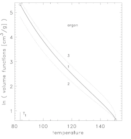
_l, and at the critical point it yields v. Figure 4 shows the temperature dependence of d

(

µ T

) (

d p T

)

for argon and the boundaries v_v and 1

(

)

[image:12.595.178.538.76.372.2]

Figure 4. Volume function d

(

µT

) (

d p T

)

of argon versus the temperature between T_t and T_c. Curve 1 represents Equation (33), curve 2 gives the lower boundary

(

)

1

2 vv+vl , and curve 3 the upper boundary vv.

Expression (33) is the only one thermodynamically possible and it alone satisfies all known thermodynamic conditions (see Appendix).

The description of the two-phase state of the saturated fluid by the expression (33) admits further formu- lations of the two-phase equilibrium.

Relations (15) and (33) yield the result of the ambitious task of representing the phase-specific internal en- ergies in terms of phase-specific volumes and vapor pressure, i.e. measurable quantities:

(

)

(

( )

)

(

)

(

( )

)

d d

, .

ln d 1 ln d 1

v l v l

v l l v

v l v l

p T p T

v v v v

u v u v

v v T v v T

 −   − 

= − ⋅ = − ⋅

   

    (34)

The positive term

(

v_v−v_l

) (

ln v v_{v l}

)

can be written in agreement with Equations (19), (20), and (33) as

(

)

.

ln

v l v v l l

v l v l

v v u v u v

v v u u

− −

=

− (35)

Rearranging this to

(

u vv v−u vl l

) (

(

uv−ul

)(

vv−vl

)

)

⋅ln

(

v vv l

)

=1 yields the following very interesting thermodynamic equations valid for T≤T_c:

ln ln 1.

v l v l v v

v l v l l v l v l l

u v v u v v

u u v v v u u v v v

       

+ ⋅ _{ }= + ⋅ _{ }=

 _{− −}   _{− −} 

        (36)

Equation (36) are valid for temperatures T =0 to T =T_c and can serve as a criterion for calculated data

,

v l

u of a gas, if the experimental data

(

u_v−u_l

)

and v_{v l,} are considered to be trustworthy. In turn, from Equa- tion (36) one obtains

(

)

, , ,

ln

v l v l

v l l v

v l v l

u u u u

u v

v v v v

− −

= −

− (37)

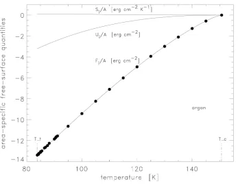
[image:12.595.214.429.81.309.2] [image:12.595.95.538.88.572.2]

[image:13.595.206.432.79.336.2]

Figure 5. Energies of saturated argon: 1 u_l, 2 u_v, 3 u,

4

(

u_l+u_v

)

, 5

(

u_l−u_v

)

.

( )

(

u vv v+ −u vl l

)

(

uv+ −

( )

ul

)

. Let us recall here the mean-value theorem of the differential calculus, which, when applied to the function ln

(

v v_{v l}

)

, yields the result

(

)

(

1

)

1

ln ln , .

ln 1

v l

v l

l v l v l v l

v v

v v

v v v ρ ρ v v v v

−

− = = −

+ − − (38)

The term

(

v_v−v_l

) (

ln v v_{v l}

)

can thus be replaced by the function v_l+

(

v_v−v_l

)

ρ, where the function

ρ

depends only on the volume ratio

(

v v_{v l}

)

or

(

v v_{l v}

)

. With the definitions

(

1

)

1 ,

(

1

)

1

ln 1 ln 1

l v

v v l v l l l v l v

v v

v v v v v v v v v v

ρ = − ₋ ρ = − ₋

    (39)

it holds that

1, 0 1 for 1.

l v l v v

v l

v l l

v v v v v

v v

v v v

ρ +ρ = ≤ρ  ρ ≤ ≥

   

    (40)

The function ρ

(

v v_{v l}

)

varies strictly monotonically from the value 1

2 at v vv l =1 to the asymptotic

value 1 for

(

v v_{v l}

)

→ ∞, the increase being greatest with 1

12 at v vv l =1, and ρ

(

v vl v

)

decreases mono- tonically to 0. The physical meaning of ρ is discussed in Ref. [16]. There the phase-specific energies u T_v

( )

and u T_l

( )

are represented as a product function, ρ⋅

(

u_v−u_l

)

, composed of the one term ρ, which denotes the phase, and the term

(

u_v−u_l

)

, which specifies the temperature dependence. The phase-specific term is related to the local interaction potential of fluid particles in the vapor space and in the liquid. With a phase change of fluid particles, the phase-specific energy value, say u_v, becomes u_l in a manner that can be des- cribed simply by interchanging the phase indices. This yields the following equations:

(

)(

)

,

(

)(

)

(

)(

)

.

v l v v l l v l l v v l v l

u =ρ v v u −u u =ρ v v u −u = −ρ v v u −u (41)

1 ln

0 1 for 1.

1 ln

v

l

u z z

z

u z z z

− −

≥ = ≥ − ≥

− − (42)

It is found that

(

u u_{v l}

)

is equal to ρ_v

(

−ρ_l

)

and varies with values between 0 and 1− as z varies from high values to 1.

The ratios of the phase-specific internal energies to the evaporation energy are likewise universal and for temperatures 0≤ ≤T T_c it holds that

(

1 ln

)

1 1

( )

(

1 ln

)

0 1.

1 2 1

l v

v l v l

u

z z z z z

u

u u z u u z

−

− − − −

≤ = ≤ ≤ = ≤

− − − − (43)

Finally, the integral Tc

(

,

)

d

Tc T v T

−

_∫

with the heat-capacity function [17] (see Figure 6),

( )

d

₍

₎

d

(

_{( )}

)

, ,

d ln d 1

v l

v l

v l

p T

v v

c T v v v v

T v v T

 −  

=  + − −  

 

  

 

(44)

yields, of course, the temperature value of the fluid internal energy,

(

,

)

(

,

)

d

₍

₎

d

(

_{( )}

)

0.

ln d 1

c

T _{v l}

v l

T

v l

p T

v v

u T v c T v T v v v

v v T

 − 

= − = + − −  ≤

 

 

∫

(45)

The entropy value s T v

( )

, is defined by the integral

(

)

0 d d d

T

s T ⋅ T

∫

because of s

( )

0,v =0. Since

(

d ds T

) (

= du dT

)

T =c T v T

(

,

)

one gets

(

)

0 d

T

s=

∫

c T ⋅ T. From this and from Equations (1) and (4) it

follows that

(

)

₀

(

,

)

( ) (

,

)

( )

d

( )

d

( )

, d .

d d

Tc T v T u T v vp T p

s T v T T v T

T T T T

µ µ

− + +

=

_∫

= = − + (46)

[image:14.595.208.425.444.686.2]

According to Equations (10), (34), and (45), one has

(

u−u_l

) (

u_v−u

) (

= v−v_l

) (

v_v−v

)

=M_v M_l . In gen- eral, it holds that [3]

Figure 6. Heat capacity c T v

(

, c

)

of saturated argon ac-