Research on neural network and application in traffic rules extraction

Journal of Chemical and Pharmaceutical Research, 2014, 6(3):204-210

Research Article

_{CODEN(USA) : JCPRC5}

ISSN : 0975-7384

Research on neural network and application in traffic rules extraction

Zhu Weiliang

1*

_{Zhang Yongli}

1

_{and Zhao Yingna}

2

1*

_{Qinggong College, Hebei United University, Tangshan, Hebei Province, China}

2

_{Hebei United University, Tangshan, Hebei Province, China}

_____________________________________________________________________________________________

ABSTRACT

This paper studied the knowledge reduction problem and discrete continuous attributes and improved the BP neural network. Firstly, methods of attribute reduction of classical are analysis. It establishes the one-dimensional cellular automata model to analyze the performance of right rule in light and heavy traffic in this paper. Subsequently, we can get the change trend of road vehicle density by the simulation of traffic flow. The data shows that the vehicle maximum density is 164veh/km. The decision rules obtained after reduction in order to map to the training sample of neural network. Finally, the simulation results show that the integration of rough set and neural network has obvious complementary and reduce the time to train the neural network.

Keywords: neural network, rules extraction, cellular automata, Lane changing model

_____________________________________________________________________________________________

INTRODUCTION

1.Background

The traffic directions of road include the right line and the lift line which is an important part in freeway traffic rules. Particularly, it has a great influence on the passing of freeway, Passing another vehicle, a very common behavior, brings the convenience for the behind vehicle. Meanwhile, there are potential dangers. Improper operation can easily lead to scratching, rollover, rear-end, which can cause obstruction for the behind to traffic. Currently, the researching of freeway direction focuses on how to determine the best passing distance. But the researching about prevailing direction and road safety issues is relatively uncommon. Therefore, we analyze the passing behavior about traffic flow and safety under the right line rules. While, we analysis the differences between the right line and the lift line.

2. Neural network

Neural network also can deal with inaccurate and incomplete knowledge. However rough sets theory and artificial neural network method of two different, rough set method to simulate human abstract thinking, neural network method is used to simulate the image intuitive thinking. Neural network general can't handle with semantic form of input rough set theory can input qualitative and quantitative or mixed information neural network can be realized without guide.

Sum up the biological neurons in the process of transfer information biological neurons is a multiple input and single output unit. When the nerve cell j has many inputsxi(i=1，2,…,m) and single outputyj, then the relationship

between input and output can be expressed as follows:

   

  



 ) ( 1

j j

j m

i ij i

j

s f y

x w

The wijis connection weights from neurons i to neurons j, and f is the transfer function or called excitation

function. After determining the neuron model, topology structure and learning method of characteristics and the ability of a neural network mainly depends on the network[1].

BP Neural network is error back propagation neural network is referred to as ", it consists of an input layer, one or more of the hidden layer and an output layer structure, each time by a certain number of neurons composition. These neurons as a man of nerve cells are interrelated. The structure as shown in figure 1 shows:

The BP neural network model

The traditional rough set of lack of semantic, rough neurons into semantic structure. Rough neural consists of a pair of overlapping normal neuron: neurons r(UpperNeural)and neuronsr(Lower Neural), neurons output outputr is always greater than the lower neuron outputoutputr:

)) ( ), (

max(f inputr f inputr r

output 

)) ( ), (

min(f inputr f inputr

r

output 

The function

f

is the transfer function in the equation.

Neural network can deal with imprecise and incomplete knowledge. However, the rough set method both theory and artificial neural network simulation method is different, the abstract thinking of human rough set, neural network method simulation image intuitive thinking. It has different characteristics[2].

The basic BP algorithm includes two aspects: the counter-propagating signals prior to the dissemination and error. The calculation of actual output from input to output direction, while the weights and thresholds of correction from the output to the input direction.

① Forward propagation process signal

The inputnetiof the firstinode in hidden layer as follows:

1

M

i ij j i

j

net w x











The outputyiof the firstinode in hidden layer as follows:

1

(

)

(

M

)

i i ij j i

j

y



net



w x













The inputnetkof the firstknode in hidden layer as follows:

1 1 1

(

)

q q M

k ki i k ki ij j i k

i i j

net

w y

a

w



w x



a

  

















The outputokof the firstknode in hidden layer as follows:

1 1 1

( ) ( ) ( )

q q M

k k ki i k ki ij j i k

i i j

o  net  w y a  w w x  a

  

 

    _   _

 







Back propagation error, namely first by the output layer to output error calculation of each layer of neurons, and then to adjust the weights of each layer and the threshold error gradient descent method, so that the final output of the modified network can meet its expected value.

For the two type of error criterion functionEpof each samplepas follows: 2

1

1

( )

2 L

p k k

k

E T o









The total system error criterion function on the training sample is as follows:

2

1 1

1

( )

2 P L

p p k k p k

E T o

 







Additional momentum method with the help of network in the correction of the weight, not only consider the role of error in the gradient, and considering the changing trends in the error surface. In the absence of additional momentum effect, the network may get into local minimum shallow value, using the additional momentum effect may be over these minima. The method is every weight in based on back-propagation method on changes on a proportional plus on previous weight or threshold changes in the amount of value, and to generate new weights based on the back propagation method or threshold changes. With additional momentum factor weights and threshold adjustment formula:

) ( )

1 ( ) 1

(k mc p mc w k

wij    i j  ij

 

Where k is the number of training and MC is the momentum factor and generally around 0.95.

3.The models to Analyze Performance of the Rule

Aiming at the time issues while drivers drive, we take NS model of cellular automaton model-one-dimensional cellular automaton model. Because cellular automaton can describe non-linear phenomena, meanwhile traffic flow is a discrete system actually; it’s uniquely superior to take the discrete cellular automaton to describe actual traffic phenomena. And since NS model is an improved model of the first cellular automaton traffic flow model, this issue can be solved well.

3.1NS Model for traffic flow analysis

In NS model, the lane is dispersed to equidistant one dimensional lattice, and numbers all vehicles from left to right. In each time step, location of vehicles is adjusted according to the speed of vehicles. Considering that vehicles have different speed in real process, the vehicles speed is taken as integer between

0

~

v

_max . At first N vehicles distribute randomly on the one dimensional discrete chain of lattice whose length is L, and each point can be occupied at most only by one vehicle. Suppose that

x

_n

，

v

_n are respectively the nth vehicle’s location and speed,

n n n

x

x

d



_1



is the distance between the n+1th vehicle and the nth vehicle at t. in each unit time step, the nth vehicle will make displacement

d

_n





v

_n



t



v

_n, N vehicles will evolution by following rules below .

①Speeding-up rule

If

v

_n



v

_max，then the nth vehicle’s speed will plus one. While if

v

_n



v

_max，then

v

_nwill not change，namely

)

,

1

min(

v

v

_max

v

_n



_n



②Speeding-cut rule under the influence of other vehicles

If

v

_n



0

， then

d

_n



d

_n



，then the nth vehicle’s speed is

(

d

_n



1

)

/



t

，namely

v

_n



min(

v

_n

,

(

d

_n



1

)

/



t

)

.

③Randomly speed changing rule by probability p

If

v

_n



0

，then the nth vehicle’ speed will minus one by probability p. while if

v

_n



0

，then

v

_nwill not change， namely

v

_n



max(

v

_n



1

,

0

)

④Location updating rule, namely

x

_n



x

_n



v

_n



t

takes the average velocity speed 120km/h while vehicles smoothly driven. Every time step stands for actual time 1s [3]

Four-step rule in NS model is the most basic rule to describe traffic flow phenomena. The first step reflects the maximum speed that drivers could make.

The second step states mutual effect between vehicles, every vehicles adjust speed according to interaction with neighbors.

The third truly reflects that different drivers have different behavior pattern in real traffic flow system. NS model proves that just because of the probabilistic speeding up or a sudden speeding cut of drivers, a traffic jam comes into being.

The fourth step reflects that the change of vehicles’ location in real traffic flow system.

3.2Solution of traffic flow NS model

We consider the time that the single vehicle A (chaser, position of the left figure 2) takes to catch the target vehicle B (being chased, position of the right figure 2) in the NS model. Making a simulation experiment with Matlab, vehicle A has two basic properties: location and speed. Speed relates to the number of vehicles on the road, so we simulate the time that the single vehicle A catch the target vehicle B in different vehicle density, at the same time, combined with the vehicle deceleration probability of random. Simulation of vehicle catching up with the target vehicle B time[4].

Fig1 The simulation test of the initial state

Fig2 Vehicle A has caught up with the target vehicle B

Blue line is the number of vehicles on the lanes, and the red line is the location of vehicle A, the target vehicle B is at the right, as long as the red line reaches to the right which represents that the single vehicle A catches up with the target vehicle B.

[image:5.595.153.449.77.322.2]

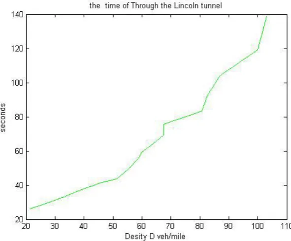
Fig.3 Time to catch up with the trend of increasing vehicle density map

We take the length of the tunnel Lincoln as the length of the highway we travel, and set the length of the path L as 480 lattice, different vehicle number randomly distribute within the road lattice, as shown in figure 1. After the beginning of the experiment, vehicle A update its attribute values in accordance with the rules, and its maximum speed is vmax = 120 km/h.

Figure 3 shows that with the increase of vehicle density and the time of vehicle, a caught up with the target vehicle B is raising. What’s more, the Curve like J-curve。In the traffic flow point of view: the more time from A after B, then through the car number is bigger also. but it can not explain the traffic flow magnitude. For illustrate this problem，We refer to the U.S. Bureau of public Roads(BPR). The function is

]

)

/

(

1

[

0





P

C

t

t





Where

t



section block time(min)



0

t

Zero flow blocking time(min)



P

Road vehicle traffic volume(veh/h)



C

Road traffic capacity(veh/h)

Fig6 This relationship between

k

_jand

c

So when the traffic density increases, the traffic flow is not necessarily increase. Such as the situation of the part of

k

_j to

k

_max in the Figure. However in 1963, Green shields proposed the linear expression of the relationship between velocity and density.

K

K

u

u

K

u

f f f





)

(

(1)

And we know the relation between velocity, flow and density.

k

u

q





(2)

Where

u

is the road speed;

u

_f is the running speed in the free flow state;

K

is the traffic density;

K

_j is the traffic density when the road becomes congestion and the flow speed is zero;

q

is the traffic flow.

Through expressions (1) (2) ,we can get the expressions of flow and density.

2

)

(

K

K

u

K

u

K

q

f f f





(3)

for the above expression



0

dk

dq

，we get

u

u

_f

2

1



，

K

K

_j

2

1



，the expression（3）has maximum value.

f f

K

u

C

4

1



(4)

Where

C

is the traffic capacity

We change the speed-density expression（1）into

)

(

u

u

u

K

K

_f

f j

_



(5)

Put expression (5) into (3) and get the flow-speed expression

u

K

u

u

K

q

_j

f j

_

Assuming the length of road

a

is

l

, we will have

f

u

l

t

₀



，

t

l

u



(7)

Where

t

₀is the road

a

running time in the free flow state

Put expression (7) into the flow-speed expression(6),and get

）

（

8

4

)

(

4

)

1

(

1

)

1

(

)

1

(

)

(

2 2 2 0 2 0

t

t

C

t

t

C

t

u

K

u

t

u

K

u

t

l

K

t

l

u

K

q

_{j f}

f f

j f j

f

j

_

_

_

_

_

_

_





A data shows that the vehicle maximum density is 164veh/km. We use the numerical density of vehicles to distinguish between light and heavy two kinds of road conditions.

Fig7 The relation curve between the traffic flow and vehicle density

Summary

Pretreatment of the sample data, reduction of attributes of the samples reduces the dimension, the approximate value, to obtain the optimal reduction of decision rules. Neurons in the hidden layer of neural network and the hidden layer number in order to map to the training sample of neural network. To make neural network more logical, and reduce the time to train the neural network, improve the training accuracy and generalization ability. Considering the right driver’s performance under the light and heavy traffic, we came up with the idea of transferring a problem of car flows into a problem of chasing time. And on the basis of lane changing model of minimum safety distance, we got those specific minimum safety distances under different conditions of overtaking. Under the condition of heavy traffic, with the decrease of the safety distance between cars, the possibility of accidents increases.

REFERENCES

[1]Wenxiu Zhang et al. Rough set theory and method. Beijing: Science Press,2001.23(10):55-58 [2]Zdzislaw Pawlak, Andrzej Skowron.Information Seienees.2007.177(27): 41-73.

[3]Kaiquan Shi, Yuquan Cui.Journal of Shandong University,2004, 39(5): 52-57.

[4] Jie Zhang, Guoguang He.Journal of Wuhan University of Technology(Transportations Science & Engineering )