Scour Analysis in High Vertical Drop Shallow Using Numerical and Physical Models

(1)

International Journal of Emerging Technology and Advanced Engineering

Website: www.ijetae.com (ISSN 2250-2459, Volume 2, Issue 6, June 2012)

348

Scour Analysis in High Vertical Drop Shallow

Using Numerical and Physical Models

M. Habibi

1

_{, M.J khanjani}

2

1_M.S, 2_{PHD, Bahonar university - kerman}

Abstract - The "vertical drop Structure" is one of the basic

types used in channel system flow. Drops are used as slope breakers in some parts of channels where we encounter supercritical slopes. Scour is a dynamic phenomenon that is visible in vertical drop tail water depth. Because of complexity of Scour process and simultaneous testing of variables’ effective compliance, studies are still underway to determine the accuracy of the equations and provide possible explanation for this phenomenon. These investigations include field or laboratory experiments under special conditions where mathematical models have been often used to provide an explicit result. Using the laboratorial physical modeling, this research explores the impact of a vertical drop flow rate on the balance of forces at the scour depth below a high vertical drop . Satisparametery results have been obtained by changing several of the parameters like sediments grading, tail water depth and flow rate. In order to specify a set of effective parameters, dimensional analysis has been used to show the scour hole dimensions. Also, computer software FLOW-3D was used to simulate the numerical modeling of Scour below a high vertical drop. The data from numerical simulation is then compared with physical modeling resulting in the great compatibility and correlation.

Keywords - drop, flow-3D, Laboratorial model, Numeric

model , Scour.

I. INTRODUCTION

The vertical drop is one kind of dissipatation structures, used as slope breakers in channel. Scour is a dynamic phenomenon which is visible in vertical drop shallow. Most riverbeds are constantly exposed to changes. Flowing water causes erosion by transporting and depositing sediments in rivers, which eventually leads to a change in the riverbed level. Changes in the riverbed may consequently alter the geometry of the river. If the depth of the scour holes become significant and reach the columns foundations of river structures, it may put their stability in peril. The parameters involved in scour hole development are complex and differ from each other depending on structure types. The high vertical drop is one of the drops used in channel flows. This structure has a considerable effect on the adjustment of flow way down the slopes.

The output flow of high vertical drop has a high energy level; thus, the hydraulics engineers must prevent serious damage and immediately address the related problems by being fully aware of energy dissipation methods, the location as well as the intensity of the scour effects on structures. Because of the complex nature of such flows and their interactions with sediment beds, studying these flows is of great importance. The previous studies show that some parameters- like flow velocity, flow jet angle, sediments grading (d50), angle of sediment yields and density froud number- have considerable effects on measurement of scour depths (Salamatian 2005). Cardoso (1999), Rouse (1935), Hanterooz (1950), Blasidell (1980), Cotolas (1960) studied and developed scour equations and scrutinized parameters that influence scour hole depths[1].

In this research, a relevant physical model was firstly made at the laboratory and an experiment was carried out to investigate scour phenomenon in high vertical drop downstream. By using dimensional analysis, the parameters involved in scour hole depths were measured and by combined. Subsequently, these results were quite compatible with those obtained from applying Flow-3d software and modeling,

Considering the impacts of changes in the geometry, the best known geometrical position of flow rate designs, types of sediment grading and downstream flow depths can be obtained by running several software programs.

Hence, by preventing the mandatory use of the USBR designed limited curves, shields curve and other references, it would be possible to take one step ahead in reducing the costs, reducing and optimizing the scour as well as the volume of the sediment leaving a site.

II. DESCRIPTION OF LABORATORY

(2)

International Journal of Emerging Technology and Advanced Engineering

349

[image:2.612.63.270.194.284.2]

The hydraulic circuit, with two 18.5 cm diameter pipes and an adjustable valve, transfers water from a tank to basin entrance through a pump with 367 kg weight, 37Kw power and 67A amperage.

Fig 1. A complete 3 dimensional (3D) view of laboratory: 1-Stilling basin 2- Basin Entrance 4- Tank 5-Basin 6-Water transfer pipes from

tank to stilling basin

The main sludge pump is inside the tank and is controlled by electrical system of the laboratory. In order to minimize turbulent flow, the water in the tank first enters an entrance tank with 1.2× 2.4 m2 surface area. Then, the flow is allowed to be slowly transferred entering the stilling basin which has a surface area of 2.44×1.26 m2 through lower pipes and enters the channel in the laboratory. This channel, which is made of reinforced concrete, is 21.85 m, 0.77 m, and 0.6 m in length, width and height. After running the flow in the channel, it is transferred to the tank in the laboratory. As it can be seen in this figure, a trapezoid overflow is located in upstream and behind the overflow drop. This overflow has been used to measuring the flow rate. The width of this overflow in the drop area has been considered to be 40 cm. The upstream flow bed is covered with coarse grained sand to create a natural bed for the upstream flow.

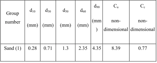
Table 1: sediments’ Grading used with their mechanical specifications Index number: the percentage passed through the screen Cu:

Coefficient of uniformity Cc: Grading coefficient

In order to check the situation of channel bed during and after each step of the experiment, the depth of sediment

scour is measured by the depth meter unit model KENEK

WH-406 with ±0.5 mm tolerance.

This device has two parts. The first part includes its main body on which the adjustments have been made (Fig.

4). The main part of this device is a monitor which shows

the measured data provided by the sensors. The collected measures (scour hole depth) are deducted from the sediment height. The second part of the device also includes a measuring sensor which contains a fixed body and an internal moving pipe (Fig. 5).

III. EXPERIMENT DESCRIPTION

[image:2.612.304.575.313.457.2]

Sediment grading experiments in sands group have been carried out and the effective parameters in soil grading like Cc, Cu, d90, d60, d50, d30 and d10 are measured and the results are shown in table 1

.

Fig. 2. shows the semi logarithmic chart of the percentage of sand sediments passed with 1.3 mm diameter.

Firstly, the experiments have been done on sands with average diameters of d50=1.3 mm and correlation coefficient of бg=3.29. If the correlation coefficient is bigger than or equals to 2 (бg≥2), the sediments aren't uniformed. Thus, the sand sediments used in this experiment aren't uniformed (3.29≥2).

After soil grading experiments, downstream sedimentary bed is prepared (as Fig. 7). Considering Fig. 7, Schoklitsch (1932) has proposed the following equation to measure scour depth:

Dse+ht= (Csq0.57H0.2)/d900.32

Cs, ht, h, q and dse are dimensional coefficient , tail water depth (m), distance between upstream and downstream (m), flow rate per unit width (m2/s) and scour depth equilibrium (m) respectively. The outflow of high vertical drop has high energy; hence, any damages and problems related to scour must be prevented through being fully aware of energy dissipation methods, scour effects on structures and location where scour occurs[2].

Group number

d10

(mm)

d30

(mm)

d50

(mm)

d60

(mm)

d90

(mm )

Cu

non-dimensional

Cc

non-dimensional

Sand (1) 0.28 0.71 1.3 2.35 4.35 8.39 0.77

0 20 40 60 80 100 120

0.1 1

10

)mm( تارذ رطق

ی

رو

بع

د

ص

رد

[image:2.612.46.297.533.634.2]

(3)

International Journal of Emerging Technology and Advanced Engineering

[image:3.612.48.283.128.273.2]

350

Fig. 3. View of high vertical drop; the important parameters are depth of tail water (ht), critical depth (yc), scour hole depth (dse), depth of tail water (yt), height of thehill (hm), scour hole depth (ds),

scour hole length (ls), all in meters and upstream flow velocity (v).

In the classification of drops, if ratio of drop height to upstream critical depth is more than 1 (H/yc)>1, it is a high drop type. To begin with, a 7.5 liter per second flow rate has been selected. This is a minimum flow rate that causes scour to start in a sedimentary bed. The experiment has been carried out in 4 stages:

1- A 7.5 liter per second flow rate and a tail water depth of 40 meters.

Firstly, water is run through a downstream channel (Fig.

2). Considering the two 40 cm and50 cm tail water depths,

when the water level becomes stable on sedimentary bed, by opening the valve in the upstream, water starts to flow over the trapezoid overflow and reaches the level of the drop overflow. At this point, falling jet into the downstream causing the scour to start (Fig. 3). In every four stage of the experiments, scour profile measurment was done five times with depth meter unit for periods of 10, 30, 60,90 and 120

minutes each time. Scour depth reached equilibrium state

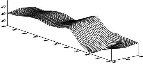
after 120 minutes continuous test run. In Fig. 8 a view of the hole and the hill has been shown created by scour at the end of the experiment.

Fig. 4. A view of the hole and the hill formed by scour at the end of the test; Points A and B indicate the hole and the created hill

respectively..

IV. ANALYZING THE TESTS RESULTS

Considering the four steps which are run through in the test description, the relevant charts and tables are submitted where dse is the depth of scour hole. 1-flow rate and depth of tail water are respectively 7.5 lit/Sec and 40 cm. 2- Flow rate is 7.5 lit/Sec and the depth of tail water is 50 cm. 3- Flow rate is 8.7 lit/Sec and tail water depth is 40 cm. 4- Flow rate is 8.7 lit/Sec and tail water depth is 50 cm.

4 se

d

(cm) (cm) 3 se

d

(cm) (cm) 2 se

d

(cm) (cm) 1 se

d

(cm) (cm) (x)(m) 3 / 01 -2 / 01 -5 / 01 -4 / 01 -01 85 / 01 -77 / 02 -0 / 03 -5 / 00 -05 4 / 02 -8 / 04 -56 / 05 -5 / 03 -21 8 / 05 -75 / 06 -06 -45 / 05 -25 3 / 04 -4 / 04 -95 / 04 -5 / 04 -31 0 / 04 -2 / 02 -12 / 03 -44 / 02 -35 0 / 02 -26 / 01 -0 / 00 -75 / 01 -41 8 / 02 -92 / 8 -9 / 9 -3 / 9 -45 3 / 9 -77 / 7 -52 / 01 -28 / 8 -51 0 / 01 -2 / 01 -02 / 00 --01 55 25 / 01 -37 / 01 -50 / 01

--01/2

61

Table 2: Variations of scour depth covering the entire length of channel (d50=1.3 mm).

[image:3.612.318.564.162.272.2]

(4)

International Journal of Emerging Technology and Advanced Engineering

[image:4.612.316.544.137.268.2]

351

Fig. 5. Variations of scour depth covering the entire length of channel (d50=1.30 mm) where the depths of tail water and flow rate are

respectively 40 cm and 7.5 lit/Sec.

Fig. 6. Variations of scour depth covering the entirelength of channel (d50=1.3mm) when the tail water depth is 50 cm and flow rate is 8.7

lit/Sec.

Fig. 7. Variations of scour depth covering the entire length of channel, d50=1.3 mm where the tail water depth is 50 cm and flow rate is 7.5

[image:4.612.47.279.147.264.2]

lit/Sec.

Fig. 8. Variations of tail water depth covering the entire length of channel where the tail water depth is 40 cm and flow rate is 8.7

lit/Sec.

In figures 9 to 12, charts related to scour profile of length of channel have been drawn at the 120th minute. In addition, by increasing the tail water depth while the flow rate is fixed, maximum depth of scour hole decreases

V. DIMENSIONAL ANALYSIS

The effective parameters on the scour hole depth (dse) at the base of a vertical drop, can be submitted as follows (2) Dse=f1(U0, y0, ht, ρ, ρs, g, ν,d50)

In the above equation, ht, ρ, ρs, g and ν are respectively tail water depth, water density, sediment density, gravitational acceleration and kinematic viscosity (10-6 m2/s ν).

∆×g parameter is introduced when the ρ, ρs and g parameters are combined (Day & Raikar 2005).

∆=s-1

The s specifies relative density of the sediment which is equal to (ρs/ρ). Also, the kinematic viscosity (ν) in a full turbulent flow on a coarse bed is simply ignored. In order to ease the dimensional analysis, methods of Buckingham & Rily as well as non-dimensional multiplication matrix method can be used.

In this research, the Buckingham method has been used. With regard to the repeated parameters U0 and y0 as well as sorting the non-dimensional parameters, the following equation is obtained in these studies

(3) dse= f2 (F0, d, h)

-18 -16 -14 -12 -10 -8 -6 -4 -2 0

0 10 20 30 40 50 60 70

)cm (لاناک لوط

)cm

(

یگ

تس

ش

با

ق

مع

-18 -16 -14 -12 -10 -8 -6 -4 -2 0

0 10 20 30 40 50 60 70

)cm

(

یگ

تس

ش

با

ق

مع

-18 -16 -14 -12 -10 -8 -6 -4 -2 0

0 10 20 30 40 50 60 70

)cm

(

یگ

تس

ش

با

ق

مع

-18 -16 -14 -12 -10 -8 -6 -4 -2 0

0 10 20 30 40 50 60 70

)cm(لاناک لوط

)cm

(

یگ

تس

ش

با

قم

ع

Length of canal

D (se)

Length of canal Length of canal D

(se)

D (se)

(5)

International Journal of Emerging Technology and Advanced Engineering

352

Where dse=dse/y0, the Froud density number is Fr0=U0/(∆gd50)0.5, d=d50/y0 and h=ht/y0.

By using laboratory data and regression analysis, the following non-dimensional equation of scour hole depth is obtained

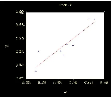
(4) dse/y0=56.82.(Fr0)-1.19.(ht/y0)- 0.21.(d50/y0)0.47 In Fig. 13 a comparing has been made between laboratory results and obtained data using equation 4.

[image:5.612.41.256.235.422.2]

.

Fig. 9. Comparison between laboratory results and obtained data using equation 4

VI. NUMERIC ANALYSIS

The Flow-3D is a powerful and highly-accurate CFD software which is designed to solve one, two and three dimensional problems (James 2003). Since this software program is established on mass principal laws as well as momentum and law of conservation of energy, it can be used to simulate various flows. One of the main capabilities of this software program for hydraulic analysis is its ability to accurately model free surface flows. The free surface is the distance between gas and liquid phases. In Flow-3D, free surface is modeled using Volume of Fluid (VOF) technique reported by Hirt & Nichds (1981). VOF method includes 3 parts:

1-Surface position display 2- Girding

3- Surface boundary conditions

VII. SEDIMENT SCOUR MODELING

The sediment scour model predicts erosion,

sedimentation and deposition of sediments and can be used for every type of flow. The combination of sedimentation model assumes sediment grains as spherical and of low velocity. Sedimentation coefficient is calculated as follows (5) Df=(SCRDLA2.RHOF)/18μ

SCRDLA: Grains’ average velocity RHOF: Fluid density

μ: fluid dynamic viscosity

The lift combination of scour is an experiential learning model which is established on bed load sediment transport models

Lift velocity is calculated by the following equation (6) Lift velocity=SCRALP√(τ-τc)/ρ

SCRALP: An experiential parameter which is used for grain scouring[4],[5].

SCRRHO: Density of sediment grains (2.56 g/cm3). ρ: Density of coarse fluid

τ: Shearing stress

(7) SCRCRT. SCRDLA. g (SCRRHO-RHOF) g: Gravitational acceleration

SCRCRT: Shields critical parameter τc: Critical shearing stress

(8) μ= μ0(1-(Solid fraction/SCRFCR))-1.55 μ0= dynamic velocity of Fluid

(6)

International Journal of Emerging Technology and Advanced Engineering

353

Fig.10.a: First step; t=0 min, d50=1.33 mm, flow rate 8.7 lit/Sec, tail water depth 40 cm.

Fig.10.b: Second step; t=10 min, d50=1.33 mm , flow rate 8.7 lit/Sec, tail water depth 40 cm.

Fig.10.c: Third step; t=30 min, d50=1.33 mm, flow rate 8.7 lit/Sec, tail water depth 40 cm.

Fig.10.d: Fourth step; t=60 min, d50=1.33 mm, flow rate 8.7 lit/Sec, tail water depth 40 cm.

Fig.10.e: Fifth step; t=90 min, d50=1.33 mm, flow rate 8.7 lit/Sec, tail water depth 40 cm.

(7)

International Journal of Emerging Technology and Advanced Engineering

354

VIII. SCUSSION AND COMPARISON

After the test and numerical simulation are carried out, the results have been compared. Table 6 demonstrates the comparison made between the Flow-3D output data and laboratorial results.

dse (cm) 10(min) 30(min) 60(min) 90(min) 120(min)

Numerical model -15.475 -15.524 15.625 15.724 16.724

Experimental model -15.5 -15.55 -15.65 -15.75 -16.75

Table3: Comparison between the laboratory and numerical results of scour depth along the time, d50=1.33 mm, flow rate 8.7lit/Sec, tail

water depth 40 cm.

[image:7.612.56.280.203.299.2]

Fig.14: Comparison between the laboratory and numerical model results; d50=1.33 mm, flow rate 8.7 lit/Sec, tail water depth 40 cm.

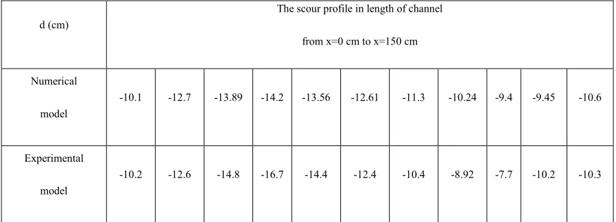
d (cm)

The scour profile in length of channel

from x=0 cm to x=150 cm

Numerical

model

-10.1 -12.7 -13.89 -14.2 -13.56 -12.61 -11.3 -10.24 -9.4 -9.45 -10.6

Experimental

model

-10.2 -12.6 -14.8 -16.7 -14.4 -12.4 -10.4 -8.92 -7.7 -10.2 -10.3

Table 4: Comparison between the laboratory and numerical model results of scour depth in the length of channel, flow rate 8.7 lit/Sec,

tail water depth 40 cm. -17 -16.5 -16 -15.5 -15 -14.5

10 30 60 90 120

)min( نامز

)

cm

(

ی

گ

تس

ش

بآ

ق

م

ع

یهاگشیامزآ لدم

یددع لدم

Physical

Numerical D

(se)

[image:7.612.82.531.343.505.2]

(8)

International Journal of Emerging Technology and Advanced Engineering

355

Dse is the scour hole depth which has been displayed in the table under specific periods of time considered .

d is the various depths which have been recorded during the formation of scour hole in the longitudinal profile area.

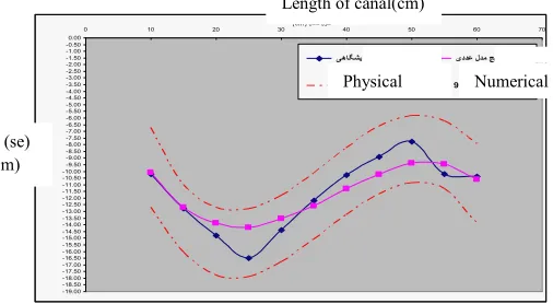
[image:8.612.29.282.253.392.2]

Considering the comparisons between the scour hole depths in the specified periods of time in table 6 as well as the comparison between the longitudinal profile in two numerical and laboratory analyses in table 7, comparison charts have been drawn in figures 14 and 15.

Fig. 15: Comparison between the laboratory and numerical model results which defines 95% prediction bounds for a new observation.

By comparing the obtained numerical model curve with the obtained curve of laboratorial model, it is observed that numerical simulation results are in prediction bounds for the laboratory determined results and show good agreement at locations.

IX. PROPOSALS

Drop structure is one of the dissipaters used in water channels. Vertical drop is one type of drops. In the design of drainage basins and drops which need a long time to reach scour depth equilibrium, predicted scour depth equilibrium is more probable than the existing equations reveals. By calculating scour depth time expansion, the amount of maximum scour depth obtained will be less. It means the scour depth should be measured in intervals between the beginning and the end of the test which will consequently reduce the costs of the construction. The greatest rates of scour occur during the first several minutes of test.

The passage of time for various flow rates causes increase in scour hole depth. While increasing tail water depth reduces the scour hole depth, decreasing tail water depth, reduces scour hole length. When the average diameter increases, the dimensions of scour hole decrease. In order to analyze the scour more accurately, better results can be achieved by comparing the laboratory results obtained from using software programs which are capable to model the scour. By using numerical model of the Flow-3D software program and a laboratory physical model, a comprehensive comparison will be made between both series of results that displays a high correlation and compatibility.

REFERENCES

[1 ] M. Shafae Bajestan (2004), "Sediment Hydraulic", Shahid Chamran

University Press, Ilam, Tehran.

[2 ] D. Taj Karimi, "Analyzing the Scour of Bed Caused by Downfall

Jets and Application of Syncretic Nerves System in that", M.A. thesis, University of Tarbiat Modarres, Technical & Engineering department, Tehran, Iran, 1998.

[3 ] J. Abrishami & M. Hoseini, "Hydraulic of Open Channels",

University of Imam Reza Press, Tehran, Iran, 2001.

[4 ] A. Azar Faradanbeh,"The Effect of Material Grading on Dimensions

of Downstream Scour Free Downfall Overflows", M.A. thesis, University of Tarbiat Modarres, Technical & Engineering department,1998.

[5 ] Bakhmeteff, B. A , Hydraulic of Open Channels, McGraw Hill, New

York, 1932.

[6 ] S. Dey &R.V. Raikar, "Scour Below High Vertical Drop", ASCE

Journal of Hydraulic Engineering, 133 ( 5), May 1, 2007 .

[7 ] J. Brethour (2003), "Modeling Sediment Scour", Flow Science, Inc

Santa Fe,NM87505.

-19.00 -18.50 -18.00 -17.50 -17.00 -16.50 -16.00 -15.50 -15.00 -14.50 -14.00 -13.50 -13.00 -12.50 -12.00 -11.50 -11.00 -10.50 -10.00 -9.50 -9.00 -8.50 -8.00 -7.50 -7.00 -6.50 -6.00 -5.50 -5.00 -4.50 -4.00 -3.50 -3.00 -2.50 -2.00 -1.50 -1.00 -0.50 0.00

0 10 20 30)cm ( لاناک لوط 40 50 60 70

)cm

( ی

گت

سش

یآ

قم

ع

یهاگشیامزآ جیاتن یددع لدم جیاتن

95% ینیب شیپ هدودحم Physical 95% ینیب شیپ هدودحم Numerical

D (se)

(cm)