Competition within random growth models

(1)

Competition within Random Growth

Models

Department of Mathematics and Statistics

Shane Turnbull

(2)

Abstract

This thesis is concerned with introducing competition into random models. It can be

observed that there are two natural mechanisms for the evolution of a random model;

either by growth or by self interactions. What we do is look at two types of models and

introduce competition within them. The first model, the voter model, is an example

of a self interacting model and we introduce growth into it. The second model, the

Hasting-Levitov model, is a random growth model and we introduce competition

within the model.

In both cases we construct diffusion approximations to model these systems when

the initial population is large for the first case and when the addition of incoming

par-ticles is small in the second. Once these diffusion processes have been constructed we

then analyse the long term behaviour of them and find their asymptotic distribution,

(3)

Dedication

Throughout my time at university there have been many people who have made here

such a fantastic experience. I have spent 8 years here at Lancaster and I am proud

to say Lancaster is my home. I shall keep the list short so apologies for not naming

many people!

Firstly, my thanks must go to my supervisor Amanda, her wisdom and guidance

has helped me throughout my time here. Apologies for all the times I turned up

unannounced at your door with a random query. I must also thank her for her

optimism for when I clearly did not have any, she always knew what to say whenever

I needed support.

I would also like to thank Tom, throughout my 8 years at university you have been

someone who I knew would be there for me, through the highs and lows your support

has always been appreciated. I know I have wasted much of your time discussing

probability theory but I hope you enjoyed some of our conversations and am glad you

have managed to retain some of it! I look forward to remaining friends even after

Lancaster, I am sure we shall.

I also extend my thanks to my family and all my friends who offered their thoughts

and encouragements while undertaking my PhD but for also offering me the distraction

during the weekends and evenings when I much needed them.

Finally, I am very grateful for the Faculty of Science and Technology for supporting

(4)

has provided me I would not have been able to do this. Thank you.

July 2018

I would also like to thank my examiners, Dmitry Korshunov and Tim Rogers, for

both their time in reading my thesis and for their invaluable comments which helped

me improve it further.

(5)

Declaration

I declare that the work in this thesis has been done by myself and has not been

submitted elsewhere for the award of any other degree.

(6)

Chapter 1 Introduction

This thesis is split into four parts, each dealing with its own specific material. Chapters

2 and 3 serve as a literature review with Chapter 2 providing a grounding in where this

area of research lies. We give a rough overview of two types of models; random growth

models and self-interacting models. As the name suggests, random growth models are

those that consist of a set which increases over time, given some probabilistic rule. We

consider the P´olya urn model since it is simple to describe and also has an asymptotic

distribution, something we are interested in with the models we consider. We also

look at the Eden model and its continuous analogue, the Hastings-Levitov model,

since part of our research focuses on this model.

Self interacting models are those that have states which change over time. We

consider the voter model, which is a simplistic model for representing the votes of

people. Again, this is another model which our research focuses on. We also include

the Moran model and that of Wright-Fisher diffusion. This is because they are both

used in population genetics where Wright-Fisher diffusion could be thought of as the

continuous limit of the Moran model. We include these here as some of our stochastic

differential equations that appear are similar to that of Wright-Fisher diffusion. We

(9)

types of behaviour.

Chapter 3 focuses on the tools required for us to construct and then analyse our

models. We start by introducing the kernel of a pure jump process. This is a very

useful object since it contains all the information of the process. With the kernel

defined we then look at what a scaling limit is and state a theorem which ensures we

have weak convergence of a sequence of stochastic processes to a diffusion process.

Once we have done this, we then analyse the obtained diffusion process. We look at

the speed measure and scale function, which are required for us to analyse our systems,

along with how to classify the boundary behaviour. This is enough information to

then find the asymptotic distribution.

The next two chapters, Chapter 4 and 5, contain our original work. We use the

tools introduced in Chapter 3 to analyse the models and work out their long term

behaviour.

Chapter 4 consists of the voter model, a self-interacting model, and we study the

behaviour after the introduction of growth. This was originally studied in [Morris

and Rogers, 2014], but we extend these results and reconfirm their results using the

kernel of a process and Kurtz’s theorem. We also give a full characterisation of the

model. We show how the addition of growth has the ability to turn absorbing states

into reflecting ones and then analyse the limiting behaviour.

In Chapter 5 we do the opposite. We consider a random growth model where the

growth is constructed via a sequence of conformal maps, in this case the

Hastings-Levitov model and introduce competition into it. We introduce a form of competition

where we allow the growth to vary depending on the harmonic measure of the regions.

We show it is necessary to allow the size and rate of the added particles to change to

(10)

Chapter 2 Random Models

The aim of this section is to give an overview of where our area of research lies. To

do this we consider two types of random models. As the name suggests, a random

model is intended to model something with a random element and is often influenced

by the world around us. There are two natural mechanisms to think of when we

consider this; growth and self-interactions. The first type of models that we consider

are those that grow, such as the Eden model. The second type of models that we

consider are those which evolve dynamically so that the states of them change over

time; an examples of this would be the voter model. After we consider these two

types of models, we consider a model that lies in the intersection of these areas; one

which grows but also evolves dynamically. This is the area that we perform research

in.

2.1 Random Growth Models

We shall consider two types of models in this section, those which grow on a lattice,

called lattice models, and those which do not, called off lattice models. Lattice models

are useful since the structure of the lattice allows us to grow clusters in an easy to

(11)

examples. Off lattice models are a better representation for real world growth, but

can be harder to model mathematically.

2.1.1 Lattice Models

In this section we look at three types of lattice models. In all cases, we are looking

at the square lattice_Z2 but these can be expanded to others.

Eden Model

A contender as a model for cell growth, the Eden model is named after Murray Eden

who studied it in [Eden, 1961] and is used to model the growth of a cluster where

the growth is motivated by the splitting of cells. Consider the square lattice with a

particle located at the origin. This has four unoccupied neighbours; we uniformly pick

one of these neighbours at random and the cell divides to occupy this cell too. This

cluster now has six neighbours and we repeat the process, letting the cluster grow,

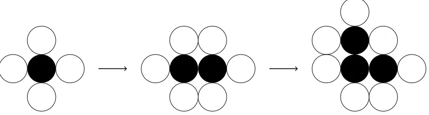
[image:11.612.113.540.456.571.2]

see Figure 2.1.

Figure 2.1: Possible first steps of the Eden model. The black cells indicate occupied sites and the white ones are the possible growth sites, which are picked with equal probability among them.

An interesting question to ask is, when we let the cluster grow for a long time, does

(12)

t→ ∞we obtain a limit object? From computer simulations [Freche et al., 1985] the

authors claim that the model does seem to exhibit anisotropic behaviour, and so is

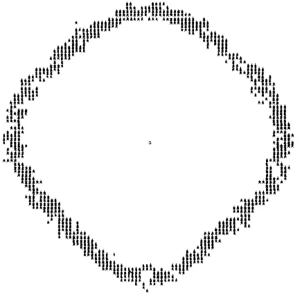
[image:12.612.219.437.151.363.2]

not isotropic, with large clusters forming a diamond shape, see Figure 2.2.

Figure 2.2: Simulation showing the anisotrophy from the growing clusters. The middle has been removed to make the boundary clearer. This is Figure 2 from [Freche et al., 1985].

Though a simple question, it was very hard to prove and very little was known

about the actual shape obtained in the limit for the first 10 years. Various attempts

have been done and some results have been gained. One of the first rigorous results

is listed below

Theorem 2.1.1. Let A be the unit circle and At the Eden cluster at time t, then

there exists aλ >0 such that for allε >0 we have, with probability 1, a large enough

t0 such that for all t > t0,

(1−ε)λA ⊂A¯t/t⊂(1 +ε)λA,

where A¯t is known as the continuum versions of At formed by replacing each point in

(13)

This result was first shown to hold in probability in [Richardson, 1973] and then

subsequently strengthened to the almost sure statement above in [Kesten, 1993]. The

main approach to showing these results is to show that the Eden model can be linked to

another model known as First-Passage percolation which we discuss in the next section

and to then show that first passage percolation satisfies a property known as

”sub-additivity”. This was generalised by Kingmann to produce the subadditive ergodic

Theorem [Kingman, 1973]. For further details see Theorem 2.1 and the surrounding

text in [Deijfen and H¨aggstr¨om, 2007].

Of course, this model can be generalised onto any graph. Consider a graph G =

(V, E) comprising a setV of vertices and E of edges. Set C0 =v0, where v0 ∈ V, to

be the initial cluster. The model grows following the iteration

Cn=Cn−1∪ {vn−1}

wherevn−1 is a vertex which neighbours the cluster Cn, which is picked uniformly at

random from all possible options.

Percolation

As the name suggests, the following model is used to represent the idea of water

seeping through a porous material. We shall restrict our study to the 2d case but this

can be extended. Imagine ann×n grid composed of 1×1 squares, with probability

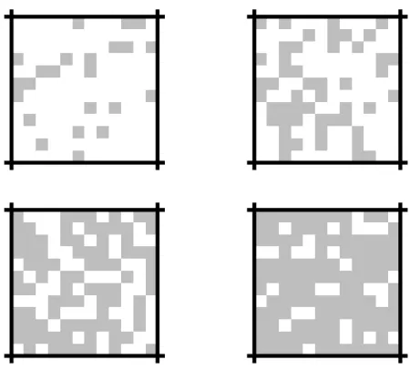
pwe let each square either be occupied or not. Some simulations for p= 0.2,0.4,0.6

and 0.8 are shown in Figure 2.3.

This model is known as site percolation since it is the sites that are being occupied,

a slight variant known as bond percolation exists where the edges of the lattice are

considered closed or open. Site percolation can be viewed as a sub-model of the

bond percolation since every bond model can be expressed in terms of a site model

(14)

[image:14.612.213.438.73.276.2]

Figure 2.3: Simulations of the percolation model for p = 0.2,0.4,0.6 and 0.8 listed from top left to bottom right. Filled in cells are coloured grey with empty ones in white.

[Grimmett, 1989]. A half way house model has been proposed called bridge percolation

which links the two, see [Chayes and Schonmann, 2000].

The first question of interest is: is it possible for the water to seep through? That

is, is there a path such that we can go from the top to the bottom? This question has

been considered in the case where the lattice in infinite in which case the question is

slightly reworded to; does there exist an infinitely large open cluster containing the

origin? This can be shown to be a probability 0 or 1 event. This in-turn raises an

observation; there must exist a critical probability, denoted bypc such that forp < pc

we will find a an infinitely large set and forp > pc we can not. In our simulations we

can see that in the case when p = 0.2 and 0.4 we can find a path but in the other

two cases there does not exist a path. This is something that has been well studied,

it was shown in 1960 by Harris that for p= 1/2 we can not find a path, see [Harris,

1960] but took another 20 years before Kesten was able to show that percolation does

not occur forp >1/2 thus showing that pc= 1/2, see [Kesten, 1980]. An overview of

(15)

As mentioned in the previous section, another model stemming from the

percola-tion model exists and is called, first passage percolation, this was first introduced by

Hammersley and Welsh [Hammersley and Welsh, 1965]. The idea is to introduce on

each site a random variable which represents the amount of time it takes for the liquid

to travel through the site, this is known as the passage time. If we denote the passage

time on site si as t(si) then the passage time of a path r which travels through the

site s1, s2, . . . , sn is just given by the sum of the passage times, that is

T(r) =

n

X

i=1

t(si).

The first passage time between two points, say uand v, is denoted byT(u, v) and is

defined to be the shortest time to travel between the two points, that is

T(u, v) = inf{T(r) :r is a path from u tov.}.

The main object of study here is following

B(t) = {v ∈_Zd_:_T₍₀_{, v}₎_≤_t}

the set of points which can be reached in time t from the origin. For further details

concerning this and percolation in general please see [Kesten, 1987].

Diffusion Limited Aggregation

We now consider another model that is similar to the Eden model, which was first

studied by Witten and Sanders in [Witten and Sander, 1983]. Once again, consider

the square lattice with an initial seed at (0,0). We start a random walk “at infinity”

and once the random walk reaches an adjacent point to the cluster it sticks. We

(16)

instead of the addition sites being chosen uniformly over all boundary points, it is now

selected with the harmonic measure of the boundary point, which is the probability

of the point being hit by the random walk. This is different from the Eden model as

in this model there is a possibility of holes being formed as they have no chance of

being filled in, whereas in the Eden model this could not happen. This model is very

hard to study and very little is known about it, a similar case holds for its continuous

variant, off lattice diffusion limited aggregation.

2.1.2 Off Lattice Models

We now look at a type of growing model that takes place in continuous space. In

the previous section, we mentioned a growth model where the growth site was picked

based on the arrival of a simple random walk. The continuous analogue to this is called

off site diffusion limited aggregation. Consider the unit disc and allow particles to

perform a Brownian path until they hit the disc, at which point they join and increase

the size of the cluster. This is very similar to the on site model, in the sense that we

have an initial site and the cluster grows randomly but with the continuous analogue

of the random walk. The probability of hitting a point is given by the harmonic

measure; this is just the probability of a Brownian particle hitting the region. In the

case of a circle, the harmonic measure is the uniform measure on the boundary. If

the shape is a simply connected object, then we can find a conformal map between

it and the circle. Since Brownian motion is invariant under conformal maps, we can

then find the hitting probabilities from the circle. This fact will be of use later.

The problem with this model is that it is very hard to say anything about it, as it

is not mathematically tractable. This is where the model proposed by Hastings and

(17)

Hastings-Levitov HL(α) Model

The model proposed is known as the Hastings-Levitov model and is one that we extend

in Chapter 5. As such, we shall dedicate this section to giving a basic understanding

of the original model. In Chapter 5, we go into more detail concerning the case when

α= 0 as this is the one we shall work with. For a more thorough introduction, please

see [Rohde and Zinsmeister, 2005].

Let K0 be the closed unit disc centered at the origin on the complex plane. We

construct a sequence of compact sets (Kn)n∈N, which represents the cluster after the

addition ofn particles. The cluster after the addition of the first particle is given by

K1 =K0 ∪P0 where P0 is the attachment of a particle at angle θ = 0. In our case,

the particle,P0, will be a slit with lengthd0, i.e. P0 = (1,1 +d0].

After the addition of the first particle, we allow particles to arrive with lengthsdn

and at angleθn. Though we talk about the slits being of lengthdn we work with what

is known as the capacity, cn, of the particles. This can be expressed as a function of

the diameter via

ecn _{= 1 +} d

2

n

4(1 +dn)

. (2.1)

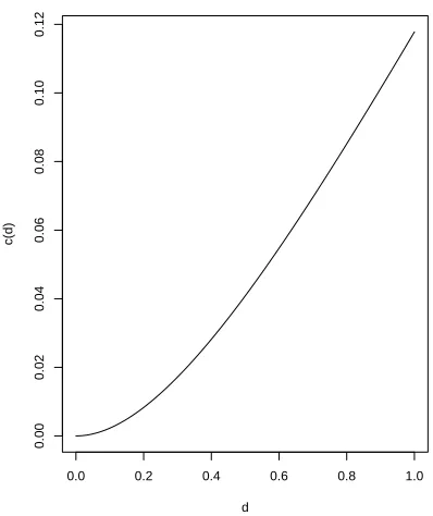
Figure 2.4 shows the relation between the values cand d, note that asc→0, d

c1/2_{. The addition of the first particle is given by the conformal map} _f _:_D

1 −→D0.

This can be constructed from a composition of conformal maps

f(z) = (m−1 ◦r◦h◦m)(z)

where

• m maps the unit circle to the real line

m(z) = iz−i

(18)

0.0 0.2 0.4 0.6 0.8 1.0

0.00

0.02

0.04

0.06

0.08

0.10

0.12

d

[image:18.612.219.418.93.330.2]

c(d)

Figure 2.4: A plot comparingc and d with relation given in Equation 2.1.

• r is a linear scaling

r(z) = _q z 1− c2

2+c2

;

• and h maps the upper half plane, minus a line

z =si:s∈

0,1₄₂₊c2_c2

2

to the upper half plane

h(z) =

c2

2 +c2

2

+z2.

Combining this, it is possible to obtain a closed form expression for the function f

[Turner, 2006].

The function f maps the exterior of the cluster unioned with a point attached at

angle θ = 0 back to the exterior of the initial cluster. This can be extended to map

the attachment of any particle at angleθ byeiθf(e−iθz).

(19)

exists a unique conformal map Φn :D0 →Dn. The map Φnis formed from a sequence

of the maps fn. This in turn will construct our sequence of growing clusters, (Kn).

Withθn representing the addition of a particle at that angle andcn being a sequence

of non-negative numbers we can generate a sequence of mapsfn and Φn

fn(z) = eiθnfcn(e

−iθn_z₎ _and _Φ

n =f1◦. . .◦fn.

In our case, the angles θn are distributed uniformly and cn = c a constant. The

Hastings-Levitov model differs from DLA since the conformal maps cause the slits to

become deformed.

The model HL(α) has the parameter α∈[0,2) which is related to the size of the

attached particle dn. The role of α is given by

dn=d

Φn−1(eiθn)

−α/2

.

Recall that cn and dn are linked by Equation (2.1) and when α = 0 we obtain the

constant case as mentioned.

Remark 2.1.1. When α = 0 the sequence of maps are independently identically

dis-tributed. This means that before we apply the conformal maps the added particles

are the same size but they become deformed after we apply the maps. Whenα = 2,

the addition of particles is changed such that, after applying the conformal maps, the

size of the particles being added is constant. The caseα= 2 is of interest since is was

thought that this could be a good model to represent DLA since in DLA the size of

the added particles are all the same, after the application of the conformal maps.

From this set up, it is now possible to analyse the system. It is shown in [Norris

and Turner, 2012] that the limiting shape is a circle. Question such as the boundary

behaviour and the anisotropic case have also been considered, see [Johansson Viklund

(20)

2.1.3 P´

olya Urn Model

There are many different types of urn models and the rules that govern them vary,

but they all follow the same set up. Suppose we start with an urn which contains

r red balls and b black balls. We operate in discrete time and at each time step

we pick a ball out of the urn, we then return that ball into the urn but also place

an additional ball into the urn of the same colour. The first question of interest is,

does such a system stabilise? That is, if we continue picking and adding balls a large

number of times, will the proportion of black and red balls converge? The answer to

this question is yes; this is easy to see as the proportion of balls is a martingale and

since the proportion of balls is bounded between 0 and 1, we can conclude that it will

converge as all bounded martingales do.

Once we know that the process converges, the next question of interest is, what

does the process converge to? If we were to repeat the process again would we

expect the process to converge to the same point or something else? In this case the

proportion of balls will converge to a distribution.

We state a more general result, intuition may suggest that if we start with an equal

number of black and red balls so that b =r then we would expect the proportion of

balls to remain 50-50. However, this is not the case, in fact, the limit is given by the

following theorem.

Theorem 2.1.2. Suppose we have a P´olya urn model withr red balls andb black balls

and at each time step we pick a ball from the urn at random. We then return the ball

and add k balls of the same colour. Let Rn and Bn represent the number of red and

black balls at timen and let Pn = _R_nR₊n_B_n be the proportion of red balls at time n, then

Pn⇒P∞ (in distribution) where P∞∼ Beta _kr,_kb

Proof. See [Mahmoud, 2009], Theorem 3.2 for further details.

(21)

the model we study in Chapter 4; the fully connected voter model when there are

no internal mechanics and growth is governed by replication. The main differences is

that the voter model is a continuous process whereas the P´olya urn model is a discrete

time model. This still enables the study of the long term behaviour via the P´olya urn

model as we shall discuss later.

As mentioned, there are many variants on the P´olya urn model. We have listed a

well known result for a generalised case when there are two balls. This model could

be extended to the case where there are a different number of colours or when balls

are returned by following a distribution.

2.2 Model with Internal Behaviour

So far we have only considered models that over time grew, we now consider another

type of model known as self-interacting models. As the name suggests, these are

models which change states over time based on the current configuration of the system.

We start this section by looking at the voter model and then consider two models

well known in the field of population genetics, the Moran model and Wright-Fisher

diffusion.

2.2.1 Voter Model

The voter model was first studied in [Clifford and Sudbury, 1973] and is a model for

the way people vote. This model allows people to vote one of two ways and allows

people to update their vote in continuous time based on the way their neighbours are

planning on voting. We describe the standard voter model, which is a generalisation

of the model we shall be working with.

Consider a connected graph G = (V, E). At each vertex there is a person who

(22)

vote with σv ∈ {−1,1}. The set of edges, e∈E, represents connections between two

people. If there is an edge linking them then they shall notify each other of how they

plan on voting and this in turn influences their vote and whether or not they will

change their vote.

In the standard model, each person changes their decision at rate 1. This can be

simulated by selecting a person at random with the time given by an exponential 1

random variable. The probability of them changing their vote is proportional to the

number of people who have the opposite view to them divided by the total number

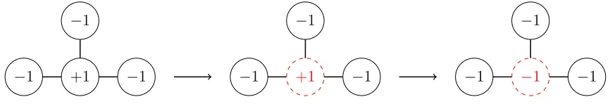
of neighbours. In Figure 2.5 we can see that the selected cell has three neighbours,

all of which share the opposite view to it and so the probability of switching is 1.

−1 +1 −1

−1

−1 +1 −1

−1

−1 −1 −1

[image:22.612.108.541.326.400.2]

−1

Figure 2.5: A person is picked at random, highlighted in dashed red and changes their vote with probability based on the proportion of votes it has from its neighbours. In this case, since all are opposite to it, they will change with probability 1.

It is clear that, given the rules of evolution, there are two invariant distributions,

when all voters agree with each other, either ±1. It can be shown that these are in

fact asymptotic distributions and, regardless of the initial configuration, will always

converge to one of these.

2.2.2 Moran Model

The Moran model, which is named after Patrick Moran, is a model for the

reproduc-tion of genes. Suppose that initially we have N genes not necessarily all distinct. At

(23)

and the other of which dies. This ensure the population remains constant and can be

thought of as two parent cells generating an offspring which inherits one of the parents

genes. In the long term it can be seen that one gene will eventually dominate and

is an absorbing state, meaning once reached we remain there. If we label the genes

1,2, . . . , N and set XN

n to be the number of type k ∈ {1,2, . . . , N} genes at time n,

then it can be seen that this is simply a Markov process with jumps ±1 or 0, as at

each time step only one cell reproduces and one cell dies. The transition probabilities

forX_nNare given by

P(XnN+1 =i+ 1|X

N

n =i) =

i(N −i)

N2

P(XnN+1 =i−1|X

N

n =i) =

i(N −i)

N2

P(XnN+1 =i|XnN =i) =

(N −i)2+i2 N2 .

This clearly shows that there are two absorbing states forXN_{, when} _XN _{is equal to}

N or 0. WhenXN ₌_N _{this represents dominance among the other genes which must}

all be equal to 0 which represents extinction. This model has been studied further

by considering whether or not the specific genes dominate. This can be studied using

knowledge of hitting times and is discussed in further detail in [Etheridge, 2011].

2.2.3 Wright-Fisher Diffusion

In the previous section we looked at the Moran model and looked at the processXN n ,

which represented the number of genes of typeN and timen. If we scale this process

by 1/N we then obtain the proportion of total genes that are of type N. If we send

N to infinity we obtain a continuous time Markov process known as Wright-Fisher

Diffusion. Such a process satisfies the following stochastic differential equation

dXt=

p

(24)

Observe that when Xt = 0 or Xt = 1 the derivative is zero, which shows they are

stationary states. It can further be shown that the process will always converge to

0 or 1. By symmetry, if the process starts at 1₂, then it must reach each point with

probability 1₂ thus making it an asymptotic distribution, see Chapter 3 and the scale

measure for further details.

What is useful about Wright-Fisher diffusion, is that it carries many of the

prop-erties of the finite Moran model but allows us to use a different set of tools to study it.

This is an example of a scaling limit, where we have changed the scale of the original

process and looked at the limiting behaviour, which is a continuous time process.

This method is useful since continuous time processes are very well understood

and have a large number of tools from Itˆo calculus to analyse them.

2.3 Random Growth Models with Competition

In this section we consider a model that lies at the intersection of the two previous

areas. That is, a model that has some form of interaction but also where the

pop-ulation size changes. We shall look at the Lotka-Volterra model which is a simple

deterministic model representing the population of two competing species.

2.3.1 Lotka-Volterra System

Consider the populations of two species of animals, one a predator, the other the prey.

As time evolves the population of these two species will evolve but will depend on

each other. As the number of predators increase the number of prey will decrease.

However, once the population of prey has decreased sufficiently, there will not be

enough food for the predator and this will cause a decrease in their population. This

will then have a knock on effect and cause the population of the prey to increase. The

(25)

Vito Volterra, who were both looking at these types of interactions. For Lotka, he

was concerned with a chemical reaction and Volterra was interested in applications in

Biology, see [Goel et al., 1971] for more details.

The System

Let x(t) and y(t) represent the number of prey and predators respectively, then the

Lotka-Volterra equations are

dxt

dt =axt−bxtyt and

dyt

dt =dxtyt−cyt

wherea, b, c, d are non-negative constants.

It can easily be seen thatxt = 0 andyt= 0 are fixed points of the above equation,

this would represent extension of both parties. There is also another fixed point to the

above pair of equations, this is given by xt = c/d and yt = a/b and would represent

steady co-existence between the two species, the rate at which they die would be equal

to the rate of birth and so we would see no change in the population.

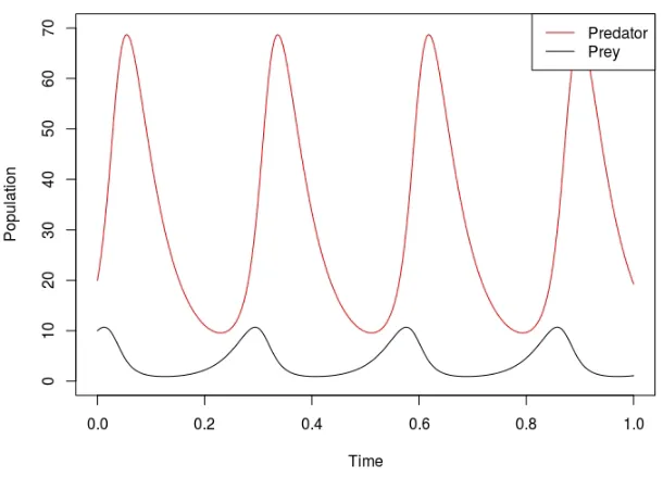
Figure 2.6 shows a numerical solution to the differential system with certain

pa-rameters. As you can see, the system appears to be periodically fluctuating up and

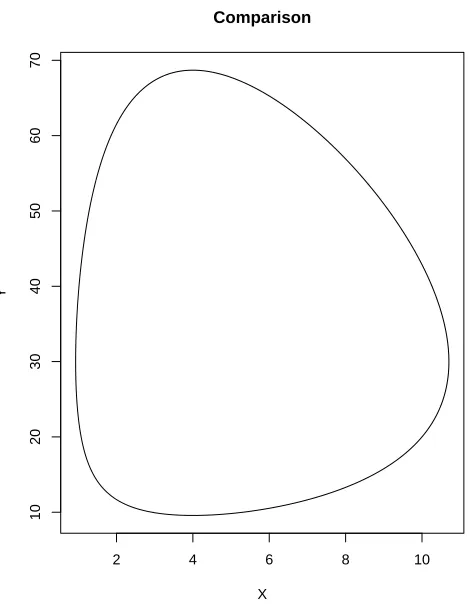
down as the other species does. Figure 2.7 highlights this periodic nature by plotting

the two populations against each other. We can see that it does indeed look periodic

and this fact is true for any values of a, b, cand d and any choice of starting points.

If we multiply and rearrange the two equations to separate the variables and then

integrate, we obtain the following

−clog(xt) +dxt=alog(yt)−byt+D,

whereD is the constant of integration. This is the equation plotted in Figure 2.7.

(26)

[image:26.612.165.470.100.320.2]

Figure 2.6: Plot of solution for a= 30, b = 1, c = 20 and d= 5.

random fluctuations, which would be expected in real life. Another shortfall of this

model is that for low values the behaviour seems unrealistic. For certain choices of the

parameters, it is possible to have the population size incredibly small, for example,

less than one. This is unrealistic since we know that a population size cannot be this

small but also, even after reaching this small size, the population still recovers and

can become large again.

Even though the model is simple, it still highlights the interest in trying to model

population size and how competition can affect this.

2.3.2 Introducing randomness

The model we have described so far is a model with growth and competition which

is something we are interested in but it does not contain any random elements. This

means we know for certain how the model will evolve over time and does not take

(27)

2 4 6 8 10

10

20

30

40

50

60

70

Comparison

X

[image:27.612.202.437.233.535.2]

Y

(28)

etc. This is one reason why this model is not a good fit to the real world. One way to

try and make the model more realistic is to allow randomness to occur, this is done

by making the process a pure jump process with the rates being motivated by the

differential equations above which describes the evolution of the system. Consider the

following system comprising of predatorsXt and preyYt which evolves like so

(x, y)→



          

          

(x+ 1, y) at rate ax

(x−1, y) at rate bxy

(x, y+ 1) at rate dxy

(x, y−1) at rate cy

The first two lines relate the the number of prey in the system and are related to

the birth and death of one respectively. The last two are the same for the predator.

Again, this system can be seen that when both are zero we have a fixed point but

now, because of the randomness we have, there cannot be any other fixed point. An

issue with the system described above is that it does allow the prey to become extinct

to which the predator will only evolve by growing, similar to the deterministic model.

Other attempts to introduce randomness into the Lotka-Volterra system have been

considered and for further reading please see [Dimentberg, 2002] and [Cai and Lin,

(29)

Chapter 3 Diffusion Theory

In the previous section we had a look at a few models; some of which were discrete

others of which were continuous. In this section, we shall look at how, from a

contin-uous time Markov chain, we can scale the process to generate a sequence of stochastic

processes such that they converge to a continuous time Markov process. The obtained

continuous Markov process will be defined via a stochastic differential equation and

we shall look at the tools required to understand such a process. We look at the

speed measure and scale function along with the Feller boundary conditions. Once

we have classified the boundary behaviour of our process we show how that is enough

to understand the long term behaviour of the process.

3.1 Motivation

Let us have a look at a simple random process which takes jumps ±1 both with rate

1 and starts at 0. Some simulations of this process are given after a different number

of steps, shown in Figures 3.1 and 3.2. As you can see, the process after 1000 steps

looks like a continuous process. This is because we have constrained the plot to fit

inside the box. A question arises though, is it possible to scale the process such that

(30)

this is yes, and there exists many theorems depending on the type of process you are

considering and the limit process you wish to obtain. In this section, we shall look at

a few that have been of use to us along with a few examples to help illustrate things.

We shall restrict our study to that of pure jump Markov processes. A pure jump

process is one whose movements are given purely by jumps and a Markov process is

one whose movement is only dependant on its current position and does not require

knowledge of the past. Though this may sound restrictive, this still incorporates a

large class of processes such as Poisson processes which are used in queueing theory

and the study of birth-death processes.

Definition 3.1.1. We say that a process Xt is a pure jump process if we can express

the evolution of the process in terms of jumps and its current location only. That is,

we can write

X→                       

X+J1(X) at rate R1(X)

X+J2(X) at rate R2(X)

.. .

X+Jn(X) at rate Rn(X)

where n is finite, Ji are the jumps of the process and Ri are the rates for the jumps

Ji respectively.

Before we consider these limit theorems though, we need to introduce one thing

that is central in the study of all these processes and this is known as thekernel. This

gives us another identical way of describing a pure jump process.

Definition 3.1.2. We say that the process Xn is a pure jump Markov process with

kernel,K, if it is a pure jump process and for all n∈_N,

P Jn ∈dt,∆XJn ∈dy|Jn> t, XJn−1 =x

(31)

0 2 4 6 8 10 12

−1.0

−0.5

0.0

0.5

1.0

1.5

2.0

Time

X_t

0 20 40 60 80 100

−10

−5

0

Time

[image:31.612.133.505.122.332.2]

X_t

Figure 3.1: Sample paths of a birth death process after 10 and 100 steps.

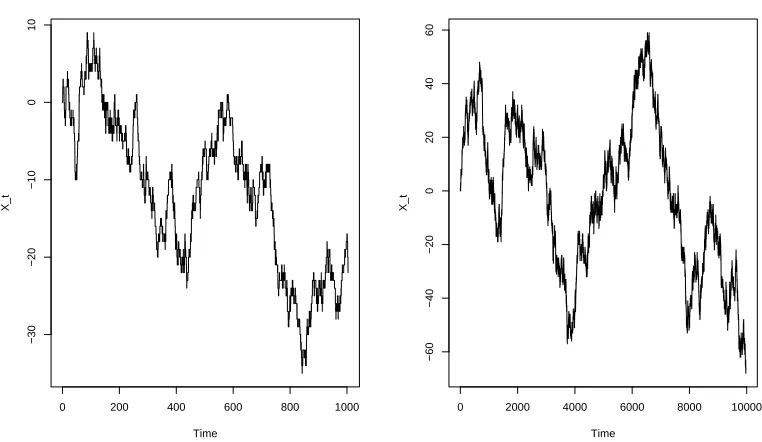
0 200 400 600 800 1000

−30

−20

−10

0

10

Time

X_t

0 2000 4000 6000 8000 10000

−60

−40

−20

0

20

40

60

Time

X_t

[image:31.612.129.510.444.665.2]

(32)

whereJ1, J2, . . . are the jump times of the process.

The kernel is useful since it contains all the information we require about the

behaviour of the process. It informs us of the probability of jumping and the direction

of the jumps.

We say that the two definitions are identical in the sense that we can derive one

from the other since they both inform us of the jumps and the rates of the process

which is all we need. We end this section with a couple of illustrative examples.

Example 3.1.1. Consider the process Xt discussed so far with jumps given by the

following,

x−→



  

  

x+ 1 at rate 1

x−1 at rate 1.

Such a process would have the following kernel associated with it,

K(x, dy) = δ1+δ−1

whereδx represents the Dirac point measure which is defined such that for a subset

A⊂_R,δx(A) = 1 if x∈A and 0 otherwise.

We can also extend the process such that it takes jumps of ±1 but this time with

rates given by λ and µ respectively. This process is known as a birth-death process.

If µ = 0, then the process is known as a pure birth process. Such a process would

have kernel given by

K(x, dy) =λδ1+µδ−1.

We now turn our attention into how we can use the kernel to show that the process,

(33)

3.2 Limit Theorem

In this section, we look at a theorem which states sufficient conditions to ensure that

the processes introduced in the previous section converges to a continuous process.

The result that we give is found in [Ethier and Kurtz, 1986] Chapter 7, though we

have altered it such that it includes the kernel directly. Similar results exist for other

types of diffusion processes, though we do not discuss them in much detail here. A

similar result for Markov chains which converge to a non-deterministic process is given

in [Gikhman and Skorokhod, 1996].

Inhomogeneous Markov Processes

The result we use is concerned with space inhomogeneous Markov processes, that is,

those processes whose movements are determined only by its current location. The

first theorem in this section will state what are the required conditions such that a

process converges weakly but before we state the theorem we need to introduce a few

concepts.

We firstly define the Skorokhod metric, this is a metric on the spaceD[0,∞). Let

Λ be the space of strictly increasing continuous functions mapping [0,∞) to itself and

let||f|| be the supremum norm, that is

||f||= sup

x>0

|f(x)|,

then the Skorokhod metric,σ(f, g), forf, g ∈D[0,∞) is given by

σ(f, g) = inf

λ∈Λmax{λ−I, f−g◦λ}

whereI is the identity function on [0,∞).

Let (XN

(34)

(respectively µ) corresponding to XN (respectively X) to be the measure defined to be

µ(A) = _P(Xt∈A) (respectively µN(A) =P XtN ∈A

)

whereA is an element of the σ−Algebra of Borel subsets of D[0,∞).

Definition 3.2.1. We say that a sequence of measures (µN₎

N∈_N converges weakly to

µif for all continuous bounded functionals f on D[0,∞) with the Skorokhod metric

we have

lim

N→∞ Z

f(x)µN(dx) = Z

f(x)µ(dx).

If this is the case, we shall write µN ⇒µ (or XN ⇒ X). Further details concerning the notion of weak convergence and the Skorokhod metric can be found in [Billingsley,

1968], Chapter 1 Section 5 and Chapter 3 Section 14 respectively.

Also the notion of Brownian motion will be of use throughout the rest of this thesis

and so we include it here.

Definition 3.2.2. A stochastic processBtwhich has the following properties is known

as Brownian motion:

• For any s < t < u < v the incrementBt−Bs is independent of Bv−Bu.

• For any s, t >0,Bs+t−Bs is normally distribution with mean 0 and variancet.

• The process Bt has almost surely continuous sample paths.

When B0 = 0 then we shall refer to it as the Standard Brownian Motion.

The following theorem is what shall be key in our study of Markov processes to

obtain a scaling limit. We shall firstly state it in the way it shall be used but this is

not how it is stated in [Ethier and Kurtz, 1986]. After stating the theorem we shall

(35)

Theorem 3.2.1. Let a = (ai,j) be a Lipschitz continuous, symmetric, non-negative

definite d×d matrix valued function on_Rd and let b:_Rd−→_Rd _{be Lipschitz}

contin-uous. Let KN(x, dy) be the kernel associated with the process XN, which takes values on some subset I ⊆_Rd _{and define}

bN(x) = Z

Rd

yKN(x, dy) and aN(x) = Z

Rd

yyTKN(x, dy).

Suppose that,

sup

x∈I

|aN₍_x₎₋_a₍_x₎_|→₀ _and _sup x∈I

|bN₍_x₎₋_b₍_x₎_|→₀

and that

sup

t>0

|XN t −X

N t−|→0 as N → ∞. If XN

0 = X0, then, setting σ2(x) = a(x), XtN → Xt weakly in D[0,∞)

where Xt is a solution to the stochastic differential equation given by

dXt=b(Xt)dt+σ(Xt)dBt.

where Bt is the standard one dimensional Brownian motion.

We now state the original Theorem and Corollary as stated in their book. Though

their terminology and notation is slightly different we will explain how it relates to

the theorem we use above.

Theorem 3.2.2 (Theorem 4.1 [Ethier and Kurtz, 1986]). Let a = (ai,j) be a

con-tinuous, symmetric, nonnegative definite, d×d matrix valued function on _Rd _{and let}

b:_Rd_−→

Rd be continuous. Let

(36)

where

Gf = 1 2

X

aij∂i∂jf+

X

bi∂if

and suppose that the C_Rd[0,∞) martingale problem for A is well-posed. For n =

1,2, . . ., let Xn _and _Bn _{be processes with sample paths in} _D

Rd[0,∞), and let An =

(An

i,j) be a symmetric d ×d matrix-valued process such that Ani,j has sample paths

in D_R[0,∞) and An₍_t₎₋ _An₍_s₎ _{is nonnegative definite for} ₀ _≤ _{s < t}_{. Set} _Fn t =

σ(Xn₍_s₎_{, B}n₍_s₎_{, A}n₍_s_{) :}_s_≤_t₎_.

Let τn

r = inf{t:|Xn(t)|≥r or Xn(t−)≥t} and suppose that

Mn ≡Xn−Bn

and

M_inM_jn−An_i,j, i, j = 1,2, . . . , d,

areFn

t -local martingales, and that for each r >0, T >0, and i, j = 1,2, . . . , d

lim

n→∞E "

sup

t≤T∧tn r

|Xn₍_t₎₋_Xn₍_t−₎_|2

#

= 0 (3.1)

lim

n→∞E "

sup

t≤T∧tn r

|Bn₍_t₎₋_Bn₍_t−₎_|2

#

= 0 (3.2)

lim

n→∞E "

sup

t≤T∧tn r

An_i,j(t)−An_i,j(t−)

2

#

= 0 (3.3)

sup

t≤T∧τn r

B_in(t)−

Z t

0

bi(Xn(s))ds

→0 in probability (3.4)

and

sup

t≤T∧τn r

An_i,j(t)−

Z t

0

ai,j(Xn(s))ds

→0 in probability. (3.5)

Suppose that P Xn(0)−1 ⇒ ν ∈ P(Rd). Then (Xn) converges in distribution to the

(37)

In essence the above theorem states that if for a given sequence of processes (Xn) you can find functions a and b such that they satisfy the above conditions, then

the sequence (Xn) converges weakly to the process X which satisfies the stochastic differential equation given by

dXt=b(Xt)dt+σ(Xt)dBt.

This is precisely what is means to be a solution to the martingale problem. The

problem arises with how to find the functions a and b. This is where the corollary is

of use.

Corollary 3.2.1 (Corollary 4.2 [Ethier and Kurtz, 1986]). Let a, bandA be as in the

previous theorem and suppose the martingale problem for(A, ν)has a unique solution

for each ν ∈ P(_Rd). Let µn(x,Γ), n = 1,2, . . . , be the transition function on _Rd, and set

bn(x) = n

Z

|y−x|≤1

(y−x)µn(x, dy) and

an(x) = n

Z

|y−x|≤1

(y−x)(y−x)Tµn(x, dy).

Suppose for each r >0 and ε >0.

sup

|x|≤r

|an(x)−a(x)|→0,

sup

|x|≤r

|bn₍_x₎₋_b₍_x₎_|→₀

and

sup

|x|≤r

nµn(x,{y:|y−x|≥ε})→0. (3.6)

Let Yn _{be a Markov chain with transition function} _µn₍_x,_Γ) _{and define} _Xn₍_t_{) =}

(38)

the martingale problem for (A, ν).

The above corollary states that from the kernel we can construct functions anand

bn_{and if these function converges to}_a_and_b _{then subject to some other conditions we}

have weak convergence. The reason we do not go into much further detail concerning

the other conditions is because they are automatically satisfied for us in all our cases.

The condition given by equation (3.6) is a requirement that the jump sizes of the

process Xn _{decrease as we increase} _n_{. The other condition given by} _{P Y}

n(0)−1 ⇒ ν

is stating that the initial distributions must converge which in our case holds since

they are all equal. The only other difference between this corollary and our theorem

is that we useKn₌_nµn

Proof of Theorem 3.2.1. See Theorem 7.4.1 and Corollary 7.4.2 in [Ethier and Kurtz,

1986].

In the previous theorem, the functions b(x) and a(x) can be thought of as the

infinitesimal drift and diffusivity of the processXtrespectively. This is why we require

the functions bN(x) and aN(x) to converge. We also require the jump sizes to tend to zero which is clearly necessary. Our final requirement is that the starting points

of all the processes coincide, this can be relaxed such that the starting points follow

a distribution and that this sequence of distributions must converge to the starting

distribution of Xt. We do not include it here since it will not be of need to us. We

shall now give a few examples where we can use the above theorem.

Example 3.2.1. Consider the birth death process given in Example 3.1.1. If we

construct the processX_tN := √1

N XN t then this would have kernel

KN(x, dy) = N δ_√−1 N

(39)

which yield the functions

bN(x) = 0 =b(x) and aN(x) = 1 =a(x)

hence, by tending N → ∞ we see that the jump sizes tend to zero. Assuming that

X₀N =X0, we can conclude, by Theorem 3.2.1, that the process XtN converges to the

process Xt which satisfies the stochastic differential equation

dXt = 0dt+ 1dBt,

which in other words means that the process Xt =Bt, a Brownian path.

Example 3.2.2. Consider again the birth-death process given in Example 3.1.1 but

with λ(x) = x and µ = 0. Such a process is known as a pure birth process; since

µ= 0, the process can only increase. This is an example of an inhomogeneous space

process since the λ depends on the location of the process Xt. The process is still

a Markov chain as we only require knowledge of its current position. Consider the

process X_tN = _N1XN t, this has the kernel

KN(x, dy) = N xδ1 N

which yields the equations

aN(x) =x=a(x) and bN(x) = 0 =b(x).

Again, the jump sizes decrease to zero as we increaseN and we make the assumption

that X0 =X0N for all N. Combining this, by Theorem 3.2.1, we obtain the ordinary

differential equation given by

(40)

which can be solved to giveXt=X0et.

One question that the above theorem does not answer is: though we know that

we have convergence of the process, what is the speed at which it converges? This

can be useful at times since this helps us obtain the error when approximating for

finiteN or when running simulations. In the case where the limit is deterministic, as

in Example 3.2.2 we can apply what is known as the fluid limit which shows we have

exponential convergence to the deterministic process, for further details see [Darling

and Norris, 2008].

3.3 Analysis of Diffusion Processes

In this section, we analyse the behaviour of the stochastic differential equations that

we can obtain by applying the theorem in the previous section. The main question

that we are interested in is: what is the long term behaviour of the process ast → ∞?

The process may settle down and converge to a point, it may converge to a set of points

with certain probabilities or it may not settle down at all. If the process does not

settle down, is it possible to find a distribution for X∞? To answer these questions,

it turns out that it is sufficient to know about the boundary behaviour along with

something called the speed measure. We shall look at the speed measure and see how

this is of use to us along with the scale function, this is a function which converts

suitable diffusion processes into martingales, which reduces the complexity. Once this

is done we shall use the speed measure to classify the boundary behaviour into one

of three types, either absorbing, reflecting, or inaccessible and we will then combine

(41)

Scale function

Firstly, suppose we have a stochastic processXtwhich satisfies the following stochastic

differential equation,

dXt=µ(Xt)dt+σ(Xt)dBt. (3.7)

Such a process is known as a diffusion process and the functions µand σ are known

as the drift and diffusivity respectively. As mentioned earlier, if we could reduce the

problem such that the above process, or some invertible function of the above process,

was a martingale, then we could analyse the martingales behaviour and that in turn

would tell us the behaviour of our original process.

To do this, we use Itˆo’s formula which allows us to calculate functions of stochastic

processes given in the form above. We state the theorem below

Theorem 3.3.1(Itˆo’s Formula). Let Xt be given in (3.7) and let f be a twice

differ-entiable continuous function, then

df(Xt) =

µ(Xt)f0(Xt) +

1 2σ

2₍_X

t)f00(Xt)

dt+σ(Xt)f0(Xt)dBt.

Proof. See Theorem 15.19 in [Kallenberg, 2002].

This is of use since if we have a process of the form (3.7) and we suppose that

we have a function f which satisfies the assumed conditions, we can apply f to the

process and determine it’s stochastic differential equation by applying Itˆo’s theorem

to see what the resulting process would be. If we now suppose thatf satisfies

µ(x)f0(x) + 1 2σ

2₍_x₎_f00

(x) = 0

then after Itˆo’s formula we would obtain a process which only has a diffusive part and

(42)

it by ρ. It can be shown that ρ must satisfy

ρ(x) =

Z x

0

exp

−2

Z y

m

µ(u)

σ2₍_u₎du

dy

wherem is a point in the interior of the interval the process takes, provided thatµ/σ2

is integrable. This is an assumption we shall need to make throughout since if this

does not hold we would not be able to transform the process.

After applying the scale function ρ we obtain the process Yt = ρ(Xt) which is of

the form

dYt= ˜σ(Yt)dBt

and so is a martingale.

Definition 3.3.1. Any process whose scale function is linear is said to be in natural

scale.

If the process is not in natural scale, then after applying ρ it will be. This can be

seen since any martingale is in natural scale asµ(x) ≡0. This reduces the study of

the diffusion process into that of a martingale. We now turn our attention to them.

For us to analyse martingales, we need to look at something called the speed measure.

Speed Measure

As we have shown with the use of the scale function, we can reduce any suitable

diffusion process into that of a martingale. This is useful since all martingales are

time changes of Brownian motion. This time change is given by the speed measure,

m. Combining this we obtain that

(43)

For a process of the form

dXt=σ(Xt)dBt

the speed measure is given by

m(dx) = 1

σ2₍_x₎dx.

In general, for a process of the form (3.7), the speed measure is given by

m(dx) = 1

σ2₍_x₎exp

2

Z x

0

µ(y)

σ2₍_y₎dy

dx.

The speed measure is of use since for any martingale, knowledge of the boundary

behaviour is given explicitly in terms of the speed measure. This in turn will allow

us to classify the long term behaviour of the process.

Boundary Behaviour

We now turn our attention to the boundary points of a process. Suppose we have a

process Xt which takes values on the interval [θ, λ], which may be infinite. We wish

to understand what these boundary points are. There are three types of boundary

points;inaccessible, absorbing and reflecting.

Definition 3.3.2. For a stochastic processXtwe say that an endpointθisinaccessible

if the probability of hitting it from any internal point is 0.

Remark 3.3.1. If the boundary point is ±∞ then it is inaccessible.

Definition 3.3.3. For a stochastic processXtwe say that an endpoint θ isabsorbing

if the event{Xs=θ} ⇒ {Xu =θ} for all u≥s.

Remark 3.3.2. Though we do not consider it, ifZθ has positive Lebesgue measure but

(44)

If the processes is sticky, it spends some positive amount of time at the end points

before leaving. See [Feller, 1952] for his original work.

Definition 3.3.4. For a stochastic process Xtwe say that an endpoint θ isreflecting

if the setZθ ={t≥0 :Xt =θ} is such that int(Zb) = ∅.

Informally, an end point is inaccessible if we can not reach it, an end point is

accessible and reflecting if once reached the particle is ejected out immediately and

the endpoint is absorbing if the process remains in the end point indefinitely.

If the endpoint is accessible then it must be either absorbing or reflecting, if it is

not accessible then it must be inaccessible. The following theorem helps us classify

the end points.

Theorem 3.3.2(Boundary behaviour, Feller).Letmbe the speed measure of a regular

diffusion on a natural scale in some interval I = [θ, λ], and fix any u∈int(I). Then,

(i) λ is accessible iff it is finite with R_uλ(λ−x)m(dx)<∞

(ii) λ is accessible and reflecting iff it is finite with m(u, λ]<∞.

Proof. See Theorem 20.12 of [Kallenberg, 2002].

Let us look at some examples to see how this can be of use.

Example 3.3.1. Consider the process Xt such thatX0 = 0 and the process satisfies

the stochastic differential equation given by

dXt=

p

1−X2

t dBt.

Clearly such a process must take values on the interval [−1,1] and so we wish to

understand the boundary points ±1. Firstly we calculate the speed measure, in this

case we have

(45)

It can be seen that

Z 1

u

(1−x)m(dx) =

Z 1

u

dx

1 +x <∞

but

m(u,1] =

Z 1

u

dx

1−x2 =∞

and so, from Theorem 3.3.2 the boundary point 1 is accessible but not reflecting and

so must be an absorbing boundary point. Similar calculations can be done on−1 to

show that it too is an absorbing point.

Example 3.3.2. Now consider a slight variant on the one above, consider the process

Xt which satisfies the equation

dXt= (1−Xt2)dBt.

Again, ±1 are boundary points but this time we have

Z 1

u

(1−x)m(dx) =

Z 1

u

dx

(1−x)(1 +x)2

≥

Z 1

u

dx

4(1−x) =∞

and so in this case the boundary point 1 is not accessible, similarly for -1. This is

because, as the process approaches the boundary points, the rate of change decreases

faster than the process can move and so does not reach the boundary point.

This raises the question of how quickly does the diffusive term need to go to zero

to ensure the end point in the above cases are accessible.

Proposition 3.3.1. Consider the stochastic process Xt which satisfies the stochastic

differential equation

dXt= (1−Xt2) α_dB

(46)

for α >0. Then the boundary points are accessible for α ≤1/2 and inaccessible for

α >1/2.

Proof. Since the process is in natural scale it is clear to see that the speed measure is

m(dx) = (1−x2)−2αdx. Applying Theorem 3.3.2 (i) we see that theR₀1(1−x)m(dx) is finite whenα ≤1/2 and infinite otherwise. A similar argument holds for the lower

boundary point.

Example 3.3.3. Consider another variant which takes values on [−1,1]. Suppose we

have a process Xt which satisfies

dXt =−

1

2Xtdt+ p

1−X2

t dBt.

This is not in natural scale and so we cannot classify the end points directly. We must

first calculate the scale function which in this case is

ρ(x) = sin−1(x).

Considering the process Yt= sin−1(Xt) and applying Itˆo’s formula yields,

dYt=dBt⇒Yt=Bt.

Observe that this shows that the processXt= sin(Bt). Since the original process Xt

takes value on the interval [−1,1] and we are now considering the processYt, this must

takes values on [−π, π]. We firstly classify these boundary points and then this in

turn will classify those ofXt. SinceYt=Bt it can easily be verified that m(dx) = dx

the standard Lebesgue measure. This means that for the boundary pointπ we have

(47)

and so the point π is an accessible reflecting point. A similar argument shows that

−π is an accessible reflecting point. Since both these points are reflecting, when we

look atXt we can conclude that they too must be reflecting points.

We now know how to classify the end points for a wide variety of processes, but how

can we use this knowledge to work out the long time behaviour of such processes? The

next theorem is what shall be of use. Beforehand, we need the following definitions.

Definition 3.3.5. A stochastic process Xt taking values on an interval A is said to

berecurrent if for any x, y ∈A

Px(Ty <∞) = 1

where_Px is the measure associated with the processXtwithX0 =xandTy = inf{t >

0 :Xt=y}.

A recurrent process can be further split into being null recurrent or positive

re-current.

Definition 3.3.6. A stochastic process Xt taking values in A which is recurrent is

called positive recurrent if for allx, y ∈A,

Ex(Ty)<∞.

If this is not the case then the process is called null recurrent.

Definition 3.3.7. A diffusion Xt with speed measure m(dx) on an interval I shall

be called m-ergodic if it is recurrent and the limit distribution of Xt has density

proportional tom for all X0 ∈I.

We now let (,[ and [[ denote the boundary point being inaccessible, absorbing or

reflecting respectively (e.g. [[0,1] means that the point 0 is a reflecting point and 1 is

(48)

Theorem 3.3.3(Feller, Maruyama and Tanaka, Theorem 20.15 [Kallenberg, 2002]).

For any regular diffusion on a natural scale and with speed measure m, the ergodic

behaviour is the following, depending on the initial position x and the nature of the

boundaries,

1. (−∞,∞): m-ergodic if m is bounded, otherwise null-recurrent;

2. (0,∞): converges to 0 a.s.;

3. [0,∞): absorbed at 0 a.s.;

4. [[0,∞): m-ergodic if m is bounded, otherwise null-recurrent;

5. (0,1): converges to 0 or 1 with probabilities x and 1−x , respectively;

6. [0,1): absorbed at 0 or converges to 1 with probabilitiesxand1−x, respectively;

7. [0,1]: absorbed at 0 or 1 with probabilities x and 1−x , respectively;

8. [[0,1): converges to 1 a.s.;

9. [[0,1]: absorbed at 1 a.s.;

10. [[0,1]]: m-ergodic.

As such, for us to understand the long term behaviour of the process, we first

use the function ρ to transform the process into a martingale so that it is in natural

scale. We then calculate the speed measure of the process, this will allow us to

work out the behaviour of the boundary points. Once we have done that we can use

the above theorem, after applying an affine transformation, to work out what the

limiting behaviour of the transformed process is and then, using the fact that ρ is

strictly increasing (and so invertible), we can work out the limiting distribution of the

(49)

Example 3.3.4 (Example 3.3.1 Cont.). In Example 3.3.1 we showed that ±1 are

both absorbing points for the processXtsatisfying dXt=

p

1−X2

t dBt. As such, we

are in case 7 of Theorem 3.3.3, and so the probabilities are directly proportional to

the distance to the boundaries. Since our process takes values on [−1,1] we need a

linear map to map it to the interval [0,1]. In this case we have f(x) = 1₂(1 +x) and

so if our process starts atx0 ∈[−1,1] we obtain that the distributionX∞ is given by

X∞ = 

  

  

+1 with probabilty 1₂(1 +x0)

−1 with probabilty 1₂(1−x0).

Example 3.3.5 (Example 3.3.2 Cont.). Example 3.3.2 showed that ±1 are

inacces-sible for the process Xt satisfying dXt = (1−Xt2)dBt. As such, we are in case 5 of

Theorem 3.3.3, and so the probabilities are directly proportional to the distance to

the boundaries. Though they are not absorbed at the endpoints, they still converge

to these points and so we obtain the same distribution as the previous example.

Example 3.3.6 (Example 3.3.3 Cont.). For the process given as a solution to the

stochastic differential equation

dXt=−

1

2Xtdt+ p

1−X2

t dBt

we know that we have reflecting boundary points at±1, this puts us in case 10 of the

theorem. This means our process is ergodic and the distribution at infinity is given

by the arcsine distribution. This can be seen since the process, Xt above has scale

function ρ(x) = sin−1(x) giving Yt = ρ(Xt) = Bt with the boundary points for the

process Yt being reflecting. The distribution is given by the uniform distribution on

(50)

Chapter 4 Addition of Growth to the Fully

Connected Voter Model

4.1 Introduction

Discrete random dynamical systems typically evolve according to one of two

mecha-nisms: growth, in which the addition of individuals or particles are governed by some

rule; or internal dynamics, in which particles within the system interact with each

other. Examples of pure growth dynamical systems include the Eden model, 2d

per-colation and the P´olya urn model. See [Lindgren, 1963] for the original work by Eden

concerning his model, [Grimmett, 1989] for details on percolation and [Johnson and

Kotz, 1977] concerning the P´olya urn model. Examples of models with purely internal

dynamics include the voter model, which is studied in [Clifford and Sudbury, 1973] or

the Metropolis-Hastings algorithm for sampling from the Ising model (originally

pub-lished in [Ising, 1925]). In this chapter, we consider a model that incorporates both

of these mechanisms; a model that has growth and internal dynamics. The model we

look at is the fully-connected voter model with growth, which was first introduced in

(51)

consider one type of internal behaviour and two different types of growth. We extend

these results in a rigorous manner. We show how to approximate the proportion of

votes for a large initial population with a diffusion process. We also calculate the limit

distributions and show how the behaviour of states can change by increasing the rate

from constant growth to exponential growth. The case where the initial population

size is small is also discussed and we comment on how our limit distribution results

still hold for all except two cases. In the cases where it does not, we show how in

one case we obtain a system that is similar to the P´olya urn model and so the limit

distribution can be explicitly calculated.

4.1.1 The fully connected voter model with the addition of

growth

Following the set up given by [Morris and Rogers, 2014], we firstly introduce the basics

of the voter model. Consider a graph G= (V, E) comprising a set V of vertices and

E of edges. On each vertexv ∈ V there exists a discrete random variable, which we

denote as σv where σv ∈ {−1,1}. The point v represents a voter and σv is the vote

of a person on the site. The way that each person may vote is influenced by their

neighbours. We shall consider the mean-field case where everyone is connected to one

another. Since we are not concerned with the individual behaviour of each person,

but the average of them, we shall look at the proportion of votes, which we denote by

x. This is a function based upon the configurations of the votes and is defined to be

x(σ) = 1

|V|

X

v∈V

σv.

This meansx∈[−1,1] with the boundary points being achieved only when the voters

all align with the same party, either −1 or +1, respectively. We denote N = |V| to

Competition within random growth models