The Poisson quasi maximum likelihood estimator: A solution to the “adding up” problem in gravity models

Munich Personal RePEc Archive

The Poisson quasi-maximum likelihood

estimator: A solution to the “adding up”

problem in gravity models

Arvis, Jean-Francois and Shepherd, Ben

World Bank, Developing Trade Consultants Ltd.

25 October 2011

Online at

https://mpra.ub.uni-muenchen.de/34334/

1

The Poisson Quasi-Maximum Likelihood Estimator: A Solution to the

“Adding Up” Problem in Gravity Models

Jean-François Arvisa _{and Ben Shepherd}b

a. Senior Economist, the World Bank, 1818 H. St. N.W., Washington, D.C. 20433.

[email protected].

b. (Corresponding Author) Principal, Developing Trade Consultants Ltd., 260 W. 52nd St. #22B, New

York, NY 10019. [email protected]. Phone +1-646-845-9702. Fax +1-646-350-0583.

The findings, interpretations, and conclusions expressed in this paper are entirely those of the authors.

They do not represent the view of the World Bank, its Executive Directors, or the countries they

represent.

Abstract: This paper shows that the Poisson quasi-maximum likelihood estimator applied to the gravity

model produces estimates in which, summing across all partners, actual and estimated total trade flows

are identical. Other methods such as OLS do not have this desirable property. Indeed, Poisson is the only

quasi-maximum likelihood estimator that preserves total trade flows. This result is an additional reason

for preferring Poisson as a workhorse gravity model estimator.

Key Words: International Trade; Gravity Model; Poisson; Quasi-Maximum Likelihood Estimator.

JEL Codes: F10; C10.

2

1

Introduction

The gravity model is ubiquitous in the applied international trade literature. Recent contributions have

highlighted a number of shortcomings with the traditional approach of log linearization and OLS

estimation. In particular, Santos Silva and Tenreyro (2006) provide strong arguments for preferring the

Poisson quasi-maximum likelihood estimator. This paper extends their findings by highlighting another

desirable property of Poisson: it preserves total trade flows between the actual and estimated bilateral

trade matrices in a way that no other quasi-maximum likelihood estimator can. Poisson thus solves the

“adding up” problem faced by other gravity model estimators.

The paper proceeds as follows. Section 2 presents a generalized gravity model. Section 3 outlines a

simple demonstration of our proposition. Section 4 provides supporting empirical evidence, and Section

5 concludes.

2

The Gravity Model

The CES-based model of Anderson and Van Wincoop (2003) has replaced more traditional formulations

to become the benchmark gravity model in the applied international trade literature:

models exports from country i to country j to be regressed against the actual values . is

expenditure; is production; is world GDP; is bilateral trade costs specified in terms of

observables, such as geographical distance, i.e. ; and is the intra-sectoral

elasticity of substitution. Inward multilateral resistance

3

multilateral resistance captures the dependence of economy

i’s exports on trade costs across all destination markets. The w terms are weights equivalent to each

economy’s share in global output or expenditure.

To estimate the model, it is common to use exporter and importer fixed effects to control for GDP and

multilateral resistance. Thus, in all generality, the standard gravity model takes the following form:

where is a constant, is shorthand for a full set of exporter fixed effects, represents importer fixed

effects, and is a random error term that is statistically independent of the regressors, with

. This setup is very close to the more general formulations of gravity

found in the regional science literature (e.g., Roy, 2004), in which the fixed effects are interpreted

generally as capturing the “repulsive” and “attractive” forces of the exporter and the importer, and a

variety of specifications for the trade costs term are considered.

To implement equation (2) empirically, the traditional approach is to use the great circle distance

between countries as a proxy for trade costs, and then to obtain OLS estimates of the log-linearized

model :

However, Santos Silva and Tenreyro (2006) highlight two problems with this approach. First, taking the

logarithm automatically drops observations for which the reported trade value is zero. This is a

significant issue empirically, because zeros are very common.

The second problem is that OLS gives inconsistent parameter estimates if the disturbance in (2) is

4

that trade data empirically exhibit more variation (standard variation over mean) for smaller trade

values resulting in a higher variance for .

Santos Silva and Tenreyro (2006) propose the Poisson quasi-maximum likelihood estimator as a

pragmatic solution to both problems. The Poisson regression model is defined in general terms by the

discrete distribution:

The expected value and variance are the modeled exports:

The log likelihood associated with the distribution is

Zero observations can be incorporated straightforwardly in the Poisson maximum likelihood (ML)

regression. It also naturally accounts for the observed dispersion (according to (5) the coefficient of

variation goes as

.) Heteroskedasticity can be handled with a robust covariance matrix, and this

approach gives consistent estimates regardless of how the data are in fact distributed, i.e. they do not

need to be Poisson at all, nor even count data. Recent simulation evidence shows that Poisson performs

well compared with other candidate estimators from the literature (Santos Silva and Tenreyro, 2011).

The quasi maximum likelihood (QML) applicable to continuous values derives from (6) and the large

5

3

Poisson and the “Adding Up” Problem

The early gravity literature recognized an additional problem with OLS estimates of the log-linearized

model in equation (3) (Tinbergen, 1962; Linnemann, 1966): Jensen’ s inequality means that total

predicted trade exceeds total actual trade. We refer to this as the “adding up” problem, in the sense

that the sum of estimated trade flows for each exporter or importer—i.e., summing across all trading

partners in the original bilateral trade matrix —systematically exceeds the total of each country’s actual

exports or imports. In Section 4, we show that this effect is quantitatively important. An additional

desirable, and unique, property of the Poisson QML is that it solves this “adding up” problem.

We proceed as follows. First, we show that the Poisson QML implies a series of equalities between

actual and estimated total trade flows for gravity models with the classical log-linear specification. Then,

we prove the following:1

THEOREM “The Poisson quasi-maximum likelihood is the only one that equalizes the totals of actual

and modeled values for any scale invariant model.”

Scale invariant models are those for which the econometric specification includes, as in (2) and (3), a

multiplicative constant to be estimated. Models that describe additive quantities, such as trade,

production, or population, which are measured in specific arbitrary units (e.g., dollars or tons)

necessarily have this property to allow for changes of units, and furthermore “adding up” makes sense

for such variables (as opposed to ratios or ordinal variables). Linear dependence in means:

1

6

Maximizing the Poisson QML (7) on the scale yields the equalizations of total values:

The empirical literature primarily uses log linear models for which the predicted values take the form:

where is the set of independent variables and the set of regression parameters. Their QML

estimate is derived by maximizing (9) given (7), which yields the first order condition (10).

Hence not only the total flow but the weighted total (or average) of each independent variable is

preserved by the Poisson QML for any log-linear model:

For dummy variables, equation (11) means that the predicted total flow for the pair ij where a dummy is

true equals the actual one for the same subset. This yields a large set of desirable equalities. For

instance, taking exporter and importer dummies as in (2) and (3), total exports and imports by country

are preserved. If the model includes regional integration variables, regional trade is conserved as well.

The surprising and important result that actual and predicted total trade flows are exactly equivalent

7

To show that Poisson is the only (quasi-) maximum likelihood estimator that preserves total flows, we

consider a general log likelihood function of the form:

The are parameters independent of the country pairs, which we can omit without loss of generality.

Maximizing the Poisson QML (7) on the scale , yields the generalization of (7) for any pairs of actual

and predicted flow values.2 At the maximum of the likelihood function:

where

Totally differentiating (13) yields:

Since the totals are conserved for the same pair , we also have:

For these two conditions to impose no further restrictions on the model, they must be proportional (two

functional forms with the same kernel are proportional). Hence:

Integration yields:

2

8

Since is QML it should have a local maximum when the two variables are identical, thus

, and , which means that:

Integrating again yields:

That is QML again implies . Therefore:

which means that . Equation 19 therefore becomes the Poisson QML:

QED

4

Empirical Implementation

In this section, we use a simple empirical example to show that the “adding up” problem we have

identified is quantitatively important, and that Poisson indeed provides an effective solution. To do this,

we set up a gravity model using aggregate trade data for 134 importers and 227 exporters for 2009,

sourced from UN-Comtrade. We include common trade cost proxies, such as geodesic distance, and

dummies for common language, geographical contiguity, colonial links, and a common colonizer. All

geographical and historical data are sourced from the CEPII distance dataset. We also include full sets of

9

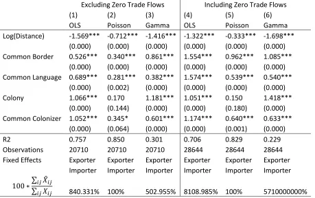
Table 1 presents results using OLS (column 1), Poisson (column 2), and Gamma (column 3), as in Santos

Silva and Tenreyro (2006). We initially consider only non-zero trade flows. In line with previous work, all

estimators provide parameter estimates that are economically meaningful and generally highly

statistically significant. However, the bottom line of the table shows that the divergence between actual

and estimated total trade flows is substantial in all cases except for Poisson, where—in line with our

theorem—the two are identical.

The same finding is apparent when we include zero trade flows in the estimation sample (columns 4-6).

(For OLS, we include zero trade flows by using as the dependent variable.) Although

parameter estimates are sensible in all four cases, the divergence between actual and estimated total

trade flows is very large for OLS, and particularly for Gamma. Again, the Poisson estimates do not suffer

from this problem, and reproduce total trade flows exactly.

5

Conclusion

This paper has demonstrated a new and desirable property of the Poisson quasi-maximum likelihood

estimator applied to the standard gravity model. In addition to dealing with heteroskedasticity and zero

trade flows, the Poisson estimator also solves what we have termed the “adding up” problem. It is the

only quasi-maximum likelihood estimator that preserves total flows between the actual and estimated

bilateral trade matrices. Our theoretical and empirical findings strengthen the case for using Poisson as

the workhorse gravity model estimator.

References

Anderson, J.E., and E. Van Wincoop. 2003. “Gravity with Gravitas: A Solution to the Border Puzzle.”

10

Linnemann, H. 1966. An Econometric Study of International Trade Flows. Amsterdam: North Holland.

Roy, J.R. 2004. Spatial Interaction Modeling: A Regional Science Context. Berlin: Springer-Verlag.

Santos Silva, J.M.C., and S. Tenreyro. 2006. “The Log of Gravity.” Review of Economics and Statistics,

88(4): 641-658.

Santos Silva, J.M.C., and S. Tenreyro. 2011. “Further Simulation Evidence on the Performance of the

Poisson Pseudo-Maximum Likelihood Estimator.” Economics Letters, 112(2): 220-222.

Tinbergen, J. 1962. Shaping the World Economy: Suggestions for an International Economic Policy. New

11

Tables

Table 1: Regression results.

Note: Prob. values based on robust standard errors adjusted for clustering by country-pair appear in parentheses. Statistical significance is indicated by * (10%), ** (5%), and *** (1%). Estimation method is indicated at the top of each column. The dependent variable is exports, except for column 1 where it is log(exports), and column 5 where it is log(1+exports).

Excluding Zero Trade Flows Including Zero Trade Flows (1) (2) (3) (4) (5) (6) OLS Poisson Gamma OLS Poisson Gamma Log(Distance) -1.569*** -0.712*** -1.416*** -1.322*** -0.333*** -1.698***

(0.000) (0.000) (0.000) (0.000) (0.000) (0.000) Common Border 0.526*** 0.340*** 0.861*** 1.554*** 0.962*** 1.085***

(0.000) (0.000) (0.000) (0.000) (0.000) (0.000) Common Language 0.689*** 0.281*** 0.382*** 1.574*** 0.539*** 0.540***

(0.000) (0.002) (0.000) (0.000) (0.000) (0.000) Colony 1.066*** 0.170 1.181*** 1.051*** 0.150 1.418***

(0.000) (0.144) (0.000) (0.000) (0.180) (0.000) Common Colonizer 1.052*** 0.345* 0.601*** 1.174*** 0.640*** 0.633***

(0.000) (0.064) (0.000) (0.000) (0.001) (0.000) R2 0.757 0.850 0.301 0.706 0.829 0.229 Observations 20710 20710 20710 28644 28644 28644 Fixed Effects Exporter Exporter Exporter Exporter Exporter Exporter

Importer Importer Importer Importer Importer Importer