Munich Personal RePEc Archive
Patterns in US urban growth
(1790–2000)
González-Val, Rafael and Lanaspa, Luis
1 November 2011
Online at
https://mpra.ub.uni-muenchen.de/34435/
Patterns in US Urban Growth (1790–2000)
Rafael González-Val, Universitat de Barcelona & IEB
Luis Lanaspa, Universidad de Zaragoza
Abstract
This paper reconsiders the evolution of the growth of American cities since 1790 in light of new theories of urban growth. Our null hypothesis for long-term growth is random growth. We obtain evidence supporting random growth against the alter-native of mean reversion (convergence) in city sizes using panel unit root tests. We also examine mobility within the distribution to try to extract growth patterns different from the general unit root trend detected. We nd evidence of high mobility when we model growth as a rst-order Markov process. Finally, using a cluster procedure we nd strong evidence in favor of conditional convergence in city growth rates within convergence clubs, which we interpret as “local” mean-reverting behaviors. We inter-pret the high mobility and the results of the clustering analysis as signs of a sequential city growth pattern.
Key words: city size, urban growth, random growth, sequential city growth, transition matrices, club convergence
JEL Classi cation: C12, 018, R11, R12
1
Introduction
This paper reconsiders the evolution of the growth of American cities since 1790 in light
of new theories of urban growth, paying special attention to sequential city growth
the-ories. The urban system of the United States (US) has often been studied because of its
special characteristics. First, it is a relatively young system (the rst census by the US
Census Bureau dates from 1790) characterized by the entry of new cities (Dobkins and
Ioannides, 2000). In addition, its inhabitants present very high mobility; Cheshire and
Ma-grini (2006) estimate that mobility in the US is 15 times higher than that in Europe. Both
characteristics, high mobility and the entry of new cities, should reduce the time transition
to spatial equilibrium between cities. In line with this, González-Val (2010) nds that the
nal decades of the twentieth century are characterized by stability in the number of cities
and the percentage of the US total population they represent, indicating a shift to a stable
city size distribution and a more consolidated urban landscape. Finally, industry cycles
have an important effect on the growth rates of American cities (Duranton, 2007). Thus, in
the second half of the nineteenth century and the early twentieth century, the growing urban
population was concentrated in the north-eastern region known as the manufacturing belt,
while in the second half of the twentieth century the rise of the Sun Belt (a phenomenon
known as regional inversion; Lanaspa-Santolaria et al., 2002) attracted population to the
West Coast area.
Many papers study the long-term evolution of American city growth. These include
Dobkins and Ioannides (2000, 2001), Kim (2000), Beeson et al. (2001), Overman and
Ioannides (2001), Black and Henderson (2003), Ioannides and Overman (2003), Kim and
Margo (2004), González-Val (2010) and Michaels et al. (2010). The spatial units (states,
counties, minor civil divisions, metropolitan areas, incorporated places, etc.) and time
periods studied and the statistical and econometrics methods used in the literature vary
widely.
the urban system in 1790. Such a wide time horizon enables us, rst, to consider the effect
of the entry of new cities (most of them during the nineteenth century), and second, to look
for different patterns of city growth. New theories have recently emerged that examine both
aspects, concluding that historically city growth may have been sequential. Sequential city
growth means that cities have early periods of fast growth (from their date of entry as a
city) followed by slow growth and/or stagnation. The idea is that during some periods,
the largest cities that entered the distribution rst are the ones that grow most. Later, their
growth slows, and the smaller cities that entered later are the ones that grow most. When
these reach a certain size, their growth rates slow again and other smaller cities are the
ones that grow fastest, and so on. It should be noted that the result is convergence among
cities. This convergence is not in size, as nal city size is determined by other factors such
as amenities, city productivity, land availability, etc., but in the growth rates at the steady
state.
Only two papers model sequential city growth: Henderson and Venables (2009) and
Cuberes (2009). The model developed by Henderson and Venables (2009) examines city
formation in a country whose urban population is growing steadily over time, with new
cities required to accommodate this growth. It yields the sequential formation of cities,
where new cities grow from scratch to a stationary size. The basic assumptions are that
city formation requires investment in xed capital in the form of housing and urban
in-frastructure and that agents are forward-looking. Cuberes (2009) presents another model
of sequential city growth; the key to generating sequential growth is the assumption of
irreversible investment in physical capital. The predictions of this second model are
empir-ically tested by Cuberes (2011), who nds strong support for sequential city growth using
two comprehensive data sets on populations of cities and metropolitan areas for a large set
of countries.
The next section presents the data used. Our basic hypothesis for long-term growth is
random growth. We use random growth as a benchmark because the effect of other
long period is considered because of the decrease in transport costs (Davis and Weinstein,
2002). Moreover, Ioannides and Overman (2003) and González-Val (2010) nd that
ran-dom growth is a good description of city size growth in the US during the twentieth century.
Therefore, in Section 3 we test random growth versus mean reversion (convergence) in US
cities using panel unit root tests. We obtain evidence supporting random growth against
the alternative of mean reversion in city sizes. In Section 4, we examine mobility within
the distribution to try to extract growth patterns that are different from the general unit root
trend. We use two different techniques. First (Section 4.1), we calculate transition
ma-trices, which tell us the degree of mobility in terms of probability, applying a generalized
equation to enable cities to enter and leave the sample. Second (Section 4.2), we apply a
cluster algorithm to identify different groups of cities that converge with each other. The
results point to a certain type of sequential growth, at least within groups. We discuss the
different empirical results in Section 5, and conclude in Section 6.
2
Data
There are various ways of de ning a “city.” The evolution of the American urban
struc-ture has been analyzed using different geographical units: counties (Beeson et al., 2001),
minor civil divisions (Michaels et al., 2010), metropolitan areas (Dobkins and Ioannides,
2000, 2001; Black and Henderson, 2003; Ioannides and Overman, 2003), urbanized areas
(Garmestani et al., 2005; Garmestani et al., 2008) or the economic areas recently de ned
by Rozenfeld et al. (2011) using the city clustering algorithm. However, since our aim is
to study the evolution of the urban system from its origin, we must use data from “legal”
cities, which are those reported since the rst census in 1790.1 Units such as metropolitan
1We talk about the “origin” of the urban system because the 1790 census is the rst one, and provides
areas were introduced later.2 Thus, we identify cities as what the US Census Bureau
de-nominates incorporated places. These places have also been used recently in the empirical
analyses of American city size distribution (Eeckhout, 2004, 2009; Levy, 2009; Giesen et
al., 2010; González-Val, 2010).
The US Census Bureau uses the generic term “incorporated place” to refer to a type of
governmental unit incorporated under state law, such as a city, town (except New England
states, New York and Wisconsin), borough (except in Alaska and New York) or village,
with legally established limits, powers and functions. We take our data from the US Census
Bureau (2004);3the sample consists of all the incorporated places with 100,000 inhabitants
or more in 2000.4
Unincorporated places (concentrations of population that form no part of an
incorpo-rated place but that are locally identi ed with a name) are excluded because they began to
be counted after 1950 (they were renamed census designated places (CDPs) in 1980).
Al-though some of them are consolidated as incorporated places and are reported in the 2000
census as cities, we also exclude them. The only exception is Honolulu CDP, because in
Hawaiian state law there are no incorporated places; they are all unincorporated.
Therefore, our nal sample in 2000 is the 190 largest cities. This sample size is similar
to that of other studies using Metropolitan Statistical Areas (MSAs). Black and
Hender-son (2003) use data from 194 (1900) to 282 (1990) MSAs, while the sample of Ioannides
and Overman (2003) ranges from 112 (1900) to 334 (1990). Their samples are slightly
2The standard de nitions of the metropolitan areas were rst issued in 1949 by the then Bureau of the
Budget, the predecessor of the present Of ce of Management and Budget.
3Source: Table 32. Only 16 of all the cities (8.42%) show a signi cant change in their boundaries (the
case of annexed areas): Anchorage, Boston, Columbus, Hampton, Honolulu CDP, Indianapolis, Jacksonville, Lexington-Fayette, Nashville-Davidson, Newport News, New York, Philadelphia, Pittsburgh, Virginia Beach, Washington and Winston-Salem. Information about entities whose names and/or boundaries have changed, entities that no longer exist, newly established entities (both legal and statistical) and changes in geographic relationships is given in the “geographic change notes” section.
4Imposing a minimum population threshold is relevant for the analysis of city size distribution (Eeckhout,
larger because in the US to qualify as an MSA a central city of 50,000 or more
inhabi-tants is needed (a lower minimum population threshold than ours). In fact, most of these
incorporated places are the central city of an MSA.
Table 1 shows the sample sizes for each decade and the descriptive statistics. For the
rst decades and until the mid-nineteenth century, the number of cities is low and grows
very slowly; however, these few cities represent about two-thirds of the total urban
popula-tion of the period. From 1850 to 1900, the number of cities doubles (from 73 to 157). The
last major entry of new cities takes place from 1900 to 1930, and from that date the number
of cities remains stable. In 2000, the percentage of the urban population represented by
this upper-tail distribution is much lower (31%) because of the appearance of many small
and mid-sized cities (there were 19,296 incorporated places in the 2000 census, with an
av-erage population of 8,968.44 inhabitants) and because a change had taken place to a more
consolidated urban landscape.
The size of our sample is an advantage from a methodological point of view because
the techniques we apply are specially designed for small samples. However, the sample is
de ned according to the largest cities in the latest period, which might imply a slight bias
because these are the “winning” cities, namely those that have presented the highest growth
rates over time. We deal with this problem in Sections 3 and 4.2 where this possible bias
could have an in uence.
3
Testing long-term trends: random growth versus mean
reversion
Description
Random growth theories are based on stochastic growth processes and probabilistic
models. The most important models are those of Champernowne (1953), Simon (1955)
these models are able to reproduce two empirical regularities that are well known in urban
economics: Zipf's and Gibrat's laws (or the rank-size rule and the law of proportionate
growth).
Random growth theory is especially important from our long-term perspective, because
the in uence of other factors such as locational fundamentals or increasing returns may
change (or even disappear) over time. Locational fundamentals are exogenous factors
linked to the physical landscape, such as temperature, rainfall, access to the sea, the
pres-ence of natural resources or the availability of arable land. These characteristics are
ran-domly distributed across space, and although they may have played a crucial role in early
settlements, one would expect their in uence to decrease over time.5 By contrast, urban
increasing returns, also known as agglomeration economies, appear later as a consequence
of industrial development. The empirical literature on agglomeration economies and their
positive effects on urban growth is wide, although there is a great deal of variability in the
results reported in the literature; see the meta-analysis by Melo et al. (2009).
Therefore, our basic hypothesis for long-term growth is random growth (or Gibrat's
law6). We follow the methodology proposed by Clark and Stabler (1991), who suggested
that testing for random growth is equivalent to testing for the presence of a unit root. They
built on the Vining model of city growth with autocorrelated errors (Vining, 1976). Let
Sit be the size (population) of cityi at time t. Starting from a simple AR growth model,
they assume that the relationship between the size of a city in time period t and t 1is
Sit = itSit 1, where itis the growth rate of cityiover the periodt 1tot. This growth rate can be decomposed into two (Clark and Stabler, 1991) or three components (Bosker et
al., 2008): a random component, a non-stochastic component relating the current growth
rate to a (possibly time-varying) constant and past growth rates, and initial city size. Then,
5However, empirical studies demonstrate that in some cases their in uence in determining agglomeration
remains important; see Ellison and Glaeser (1999) or Davis and Weinstein (2002).
6According to Gabaix and Ioannides (2004), “Gibrat's Law states that the growth rate of an economic
after some algebra Clark and Stabler (1991) get the following expression:
lnSit=ci+ ilnSit 1+
n
X
j=1
ij lnSit j+uit, (1)
whereci is a constant, ij is a parameter measuring the in uence of past growth rates on
current city growth and uit is a random error term. i is the key parameter that captures
the effect of initial city size on growth. Random growth would imply i = 0, meaning that the growth of a particular city does not depend on the initial city size. This shows that
testing for random growth (Gibrat's law) is equivalent to testing for a unit root in city sizes.
Evidence supporting a unit root (if i is not signi cantly different from zero) means that
cityi's growth rate is independent of initial size. By contrast, when i <0the evolution of city iwill be a stationary process (mean reversion).7 Using Eq. (1), Clark and Stabler
(1991) apply the standard Dickey–Fuller (1979) t-statistic, not rejecting random growth for
the seven largest cities in Canada from 1975 to 1984.
Results
Gabaix and Ioannides (2004) emphasize “that the next generation of city evolution
em-pirics could draw from the sophisticated econometric literature on unit roots.” According
to this suggestion, most recent studies apply unit root tests: Black and Henderson (2003),
Sharma (2003), Resende (2004), Henderson and Wang (2007) and Bosker et al. (2008).
Some authors (Black and Henderson, 2003; Henderson and Wang, 2007; Soo, 2007)
propose a growth equation to test the presence of a unit root, which they estimate using
panel data. However, there are problems with this methodology (Gabaix and Ioannides,
2004; Bosker et al., 2008; González-Val et al., 2010). First, data availability; we have only
22 temporal observations as the periodicity of our data is by decades (decade-by-decade
city sizes over a total period of 210 years), when the ideal would be to have at least annual
data (as Clark and Stabler, 1991, or Bosker et al., 2008). Most studies use data from
7A consequence of an estimated
the decennial census, so this limitation is a common problem in the literature. Second,
an econometric issue; the presence of cross-sectional dependence across the cities in the
panel can give rise to estimations that are not very robust. Econometric literature clearly
establishes that panel unit root and stationarity tests that do not explicitly allow for this
feature among individuals present size distortions (Banerjee et al., 2005).
For this reason, as in González-Val et al. (2010), we use one of the most recent tests
especially created to deal with this question, namely Pesaran's (2007) test for unit roots in
heterogeneous panels with cross-section dependence. The test of the unit root hypothesis
is based on the t-ratio of the OLS estimate ofbiin the following cross-sectional augmented
Dickey–Fuller (denoted by CADF) regression:
yit=ai+biyi;t 1+ciyt 1+di yt+eit, (2)
whereyit = lnSit,aiis the individual city-speci c average growth rate andytis the cross-section mean of yit, yt = N 1PNj=1yjt. To eliminate cross-dependence, the standard
Dickey–Fuller (or augmented Dickey–Fuller) regressions are augmented with the
cross-section averages of lagged levels and rst differences of the individual series, such that the
in uence of the unobservable common factor is asymptotically ltered. The null hypothesis
assumes that all series are non-stationary, and Pesaran's CADF is consistent under the
alternative that only a fraction of the series is stationary.
Another advantage of Pesaran's CADF test over other recently developed unit root tests
(Levin et al., 2002) is that it is suitable for unbalanced panels, as is the case with our city
sample8. New cities appear over time, from 16 in 1790 to 190 in 2000. However, owing to
limitations in the data (the CADF test works with unbalanced panels but if we consider the
complete sample it is a strongly unbalanced panel; there is an excessive amount of missing
8Another panel test that deals with cross-section dependence and that is suitable for unbalanced panels is
data) we must restrict our analysis to a maximum of 150 cities. These 150 cities are a xed
sample for the entire period, and correspond to the largest cities (upper-tail distribution)
in the year of reference. We consider three different periods: 1790–1900, 1900–2000 and
1790–2000. In the 1790–1900 period, the year of reference is 1860 while in 1900–2000
and 1790–2000 it is 1900 (we cannot use always the same year of reference owing to data
limitations). In this way, we can control the possible bias mentioned in Section 2, because
not all the largest cities of 1860 or 1900 would have maintained their positions a century
later. Therefore, the samples de ned according to 1860 or 1900 ranks contain “winning”
and “losing” cities.9
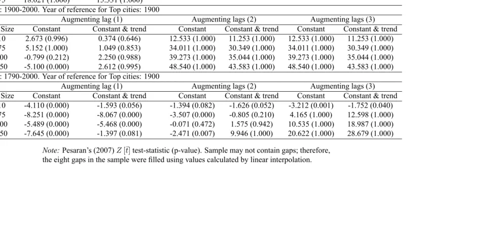
Table 2 shows the results of the standardized Ztbar statistic of the CADF test, Z[t], and the corresponding p-value for four sample groups (top 10, 75, 100 and 150 largest
cities in the year of reference), different speci cations: AR(p)withp = 1;2;3including a constant or constant and trend, and three different periods.10 In Panel A (1790–1900),
we must restrict the analysis to top 10 and 75 owing to data limitations; the results show
that we cannot reject the unit root in any case. Support for the unit root hypothesis is also
strong in Panel B (1900–2000), as we can only reject the null hypothesis in one case: the
model with one lag and no trend for the top 150 cities. Finally, Panel C, which considers
the entire period 1790–2000, shows less unanimous evidence. In this panel, the results are
similar for the four sample sizes. When only one lag is included, the null hypothesis of
9Moreover, 1900 is when our sample exceeds 150 cities (see Table 1).
10The estimations were made with the pescadf Stata package, developed by Piotr Lewandowski. The
number of cities in each panel in Table 2 is xed, although some of the cities did not exist in all periods (that is why Panels A and C are unbalanced panels). To clarify this point, these are the number of time observations for each city in the panels:
Panel A: 1790–1900. Year of reference for Top cities: 1860. Top 75 (N=75): (N, T1-T75) = (75, 11 11 11 11 9 9 7 6 9 7 11 10 5 11 10 7 8 6 8 11 11 7 7 6 5 11 11 11 5 10 11 9 6 6 7 10 11 11 6 5 6 11 6 9 5 5 4 6 5 6 10 11 6 5 6 4 5 4 5 7 4 5 6 4 5 10 4 4 5 4 5 5 4 5 5). Top 10 is the subsample with the rst 10 elements (N=10, T1-T10).
Panel B: 1900–2000. Year of reference for Top cities: 1900. This is a balanced panel; there are 11 temporal observations for each city.
a unit root is rejected for any speci cation. However, as the number of lags in the model
increases we soon nd evidence in favor of our null hypothesis: in the model with two lags
when a trend is included, and in the model with three lags with any speci cation. This last
result is especially relevant, as Said and Dickey's (1984)T1=3 rule would establish the lag
choicep= 3in that case 221=3 = 2:8 .
This evidence in favor of a unit root indicates that city growth during the 1790–2000
period was independent of initial size, supporting our hypothesis of random growth. The
evidence is even stronger when we consider subperiods (1790–1900 and 1900–2000). We
carried out several robustness checks with the Panel C sample (the whole 1790–2000
pe-riod).11 First, we de ned the sample according to the largest cities in 2000, the latest period
for which we have data. The results of the test, when it could be carried out,12were similar:
with two lags or more, we could not reject the unit root for any speci cation of the model.
We also tried de ning the group of cities randomly, and again we obtained the result that
the null hypothesis of a unit root could not be rejected (in this case, the only model with
which it could be rejected was withp= 1and without trend). Finally, we estimated sepa-rately a panel for the sample of 16 cities that are present in all periods. In this case, as we
considered a balanced panel we were also able to run the tests of Levin et al. (2002) and Im
et al. (2003). The results for this group of the oldest cities were similar; we could not reject
the null hypothesis from two lags onward with any speci cation of the model and with any
of the three tests.
4
What lies beneath the random growth? Intra-distribution
mobility
In Section 3, we found evidence supporting random growth against the alternative of mean
reversion (convergence) in American cities during the 1790–2000 period. This type of
11The speci c values of the tests are available from the authors on request.
growth pattern implies that cities evolve according to a stochastic process in which the
growth rate does not depend on the initial size, so that the differences in the nal sizes
of the cities depend on exogenously distributed characteristics (locational fundamentals
theory) or random shocks. In this case, under certain conditions the limit distribution of
city size must converge to a Pareto distribution that obeys Zipf's law (Gabaix, 1999).
In this section, we take a different perspective. Our intention is to examine mobility
within the distribution, trying to extract growth patterns different from the general unit root
trend detected in the previous section. To do this, we use two different techniques. First, we
calculate transition matrices, which tell us the degree of mobility in terms of probability.
Second, we apply a cluster algorithm to identify different groups of cities that converge
with each other. Both approaches are complementary; while the transition matrices de ne
some groups in relative terms and the movements of cities between these groups are
exam-ined, with the second method we use the algorithm to identify endogenously the groups of
cities that converge over time, looking for evidence of some type of “local” mean-reverting
behavior.
4.1
Transition matrices
Description
Eaton and Eckstein (1997) were the rst to apply Quah's (1993) transition matrices to
city size evolution. LetFt be the vector representing the city size distribution at instantt,
relative to the average size. We can say that this distribution follows a stochastic process
de ned by a Markov chain if the transition from one period to the next is given by:
Ft+1 =MtFt, (3)
whereMtis the movement matrix or transition matrix de ning the law of movement from
one period to the next. If Mt is time-invariant, then we have a stationary process and
represents a discrete approximation to population distribution. Implicit in (3) is also what
is known as the Markov property, i.e., that the future of the process depends only on its
most immediate past (a homogeneous rst-order stationary Markov process). Elementpij
of the matrixM represents the probability that a city in stateiintmoves to statejint+ 1,
i; j 2E. It is evident thatpij 0and that
P
j2E
pij = 1;8i2E.
The elements of the matrix M can be estimated by maximum likelihood (Hamilton,
1994; Bosker et al., 2008) applying:
^
pij = TP1
t=1
nit;jt+1
TP1
t=1
nit
, (4)
wherenit;jt+1 is the number of cities moving from stateiin yeart to statej in yeart+ 1
andnitthe number of cities in stateiin yeart.
The general expression (3) is valid for the case in which no cities enter or leave the
sample from one year to the next. This is not our case, and thus we need to apply an
extended equation, which describes the evolution of a distribution that allows cities to enter
or leave.
In the case of a sample that grows over time, in which from one period to the next cities
only enter, Dobkins and Ioannides (2000) and Black and Henderson (2003) show that the
correct equation is:
Ft+1 = (1 it)M Ft+itZt, (5)
where it is a scalar denoting the percentage of new cities in t+ 1 over the total existing cities int+ 1andZtis the vector of relative frequencies of the cities that enter.
In our case, where cities enter and leave the sample from one period to the next, Lanaspa
et al. (2011) propose the next equation:
where nt = NNt with N denoting the constant number of cities in each period and Nt representing the number of cities entering or leaving fromttot+ 1,Zt(Xt) is the vector of relative frequencies of the cities that enter (leave) the sample andM is the transition matrix
fromttot+ 1but only of theN Nt cities that are in the sample both int and int+ 1. The difference between Eq. (6) and Black and Henderson's (2003) expression (Eq. 5) is
the termntM Xt, which represents the distribution of cities that leave the sample.
Results
Table 3 shows theM matrices for three different periods (again 1790–1900, 1900–2000
and 1790–2000) and three sample sizes (75, 100 and 150 cities). This methodology always
takes into account the largest cities at each moment in time, allowing these largest cities
to change, enter or leave the sample, or remain in it from one period to the next. 13 Five
states are considered; a larger number would increase the mobility arti cially and a smaller
number would provide little information on intra-distribution mobility. The upper limits
for each state are 0.4, 0.7, 1, 2 and1times the average for each year.14 The thresholds of
the different categories are not exactly the same, but they are very similar to those used by
Eaton and Eckstein (1997), Dobkins and Ioannides (2000) and Bosker et al. (2008). In any
case, one of the criteria used to de ne them is that the number of cities in each of the
cate-gories should not be different. As is already known, the major problem with this approach
is that any choice of states inevitably involves a certain amount of arbitrariness. With this
in mind, we explored alternative cut-off points, although these are not very different from
the states nally chosen, and the qualitative results remain the same. The relative
frequen-cies are also shown of the cities that enter ( Zt) and leave the sample (Xt) throughout the
period, as de ned above.
Several conclusions emerge from Table 3. The rst and most important is that we nd
intense mobility in the distribution of cities; persistence is not high. This is especially true
13But to de ne the largest cities in each period, entry and exit, we use all the cities available each year.
14The average is not calculated for all the cities, but for those that remain in the sample for two consecutive
for Panel A (1790–1900), which captures the creation of cities in the nineteenth century,
and Panel C (1790–2000), which represents the aggregate period. In fact, many of the
ele-ments in the diagonal of the matrices in Panel A, which correspond to the cities that belong
to the same state for two consecutive periods, are below 0.7, thus indicating high mobility
in that period. Panel B shows less mobility, as most of the elements in the diagonal of the
matrices are greater than 0.8. These results highlight the difference between the nineteenth
(high mobility) and twentieth century (a more stable urban system). The matrices in Panel
B are consistent with those of Black and Henderson (2003), as the period they consider is
similar (1900–1990). Focusing on the aggregate period 1790–2000 (Panel C), of the fteen
elements in the diagonals, only three are higher than 0.9, while six values are between 0.7
and 0.8, and one is below 0.7. All of them are signi cantly different from one (value one
represents no transitions to any other states and thus absolute persistence).15
It is usual in the literature to nd little mobility, as detected for the US by Black and
Henderson (1999, 2003) and by Beeson et al. (2001), but those samples cover a
consid-erably shorter time horizon than the one we consider. Our sample covers more than two
centuries. By studying the urban structure from its beginning the conclusions may be
dif-ferent, because over these centuries, the late eighteenth, the nineteenth and the twentieth,
the American urban structure was formed and built through demographic expansion (waves
of immigration throughout the nineteenth century) and territorial expansion (the so-called
conquest of the West and the founding of the cities of the West and Mid-West). Other works
that consider the same time horizon (1790–2000) also nd evidence of high mobility within
the distribution (Batty, 2006; Cuberes, 2011). Thus, Batty (2006) develops rank-clocks that
show how, with the exception of New York, the cities of the original 13 colonies gradually
lost their positions with the entrance of new cities. Our data show the same behavior as a
consequence of the mobility noted above and the entry of new cities. If we rank cities in
2000 only New York, Philadelphia, Boston and Baltimore of all the cities that existed in
the rst period (1790) are still among the top 20 cities (and only New York and
phia remain within the top 10 cities), while the rest have lost their positions and have been
overtaken by other cities that entered the system later.
Cuberes (2011) nds that the average-rank of the fastest-growing cities (not just
Amer-ican cities, as his sample includes data for cities in other countries) tends to increase over
time, a result that he interprets as evidence in favor of sequential urban growth. If cities
grow sequentially, the cities that are initially the largest must represent a large share of
the total urban population of the country in the initial periods and a relatively smaller one
later on (although this is a necessary but not suf cient condition). As Table 1 shows, the
behavior of our sample of cities is consistent with this af rmation.
The second conclusion refers to the cities that enter (Zt) and leave the sample (Xt). In
the three panels, those cities that leave the sample do so almost exclusively from the fth
state, that of the smallest cities. It makes sense that large cities do not disappear suddenly.
In Cuberes (2009) and Henderson and Venables (2009), the explanation is that there is
irreversible investment. In Glaeser and Gyourko (2005), it happens because housing is a
durable good that depreciates slowly over time. This fact is not the same for cities entering
the sample; in Panels A and C they enter in all the states, except for that of the largest
cities. Nevertheless, in Panel B, which we claim represents a more stable urban structure,
cities only enter to the last two states (the smallest cities in the samples). From a long-term
perspective (Panel C), this result indicates that cities enter the sample with a considerable
size (most of them cities created in the West) and grow very quickly until they reach the
sizes of the pre-existing cities (leapfrogging).
4.2
Convergence clubs
Description
The results in Section 3 show that we cannot reject the random growth (unit root)
hy-pothesis for most of the proposed speci cations, against the alternative hyhy-pothesis of
mobility when we model growth as a rst-order Markov process. That approach explains
how cities move between the different population thresholds we de ned; however, more
or less movement does not automatically imply convergence or divergence. Therefore, in
this section we apply a cluster algorithm to try to identify different groups of cities that
converge with each other, looking for evidence of some type of “local” mean-reverting
be-havior. Cluster analysis has previously been used to study clusters of cities within city size
distribution (Garmestani et al., 2005), but here we look for clusters in city growth rates
rather than clusters in city sizes.
The cluster procedure is based on the logt test (Phillips and Sul, 2007, 2009), which
focuses on the evolution over time of the idiosyncratic transitions in relation to the
com-mon growth component. Therefore, in Section 3 we analyzed the evolution of the comcom-mon
growth component using panel unit root tests and now we focus on the possible
differ-ences in the idiosyncratic transitions across cities. This new approach is different from that
of previous empirical studies on growth convergence clubs, such as Durlauf and Johnson
(1995) and Canova (2004). The regression model of the logt test is:
logH1
Ht
2 log (logt) = 0 + 1logt+ut, fort=T0; :::; T (7)
whereH1
Ht is the cross-sectional variance ratio,Htis the transition distance,Ht=N
1PN
i=1
(hit 1)2, andhit is the relative transition coef cient, de ned ashit = logSit
N 1 N
P
i=1
logSit
(againSit is the
size (population) of cityiat timet.). These relative transition coef cients exclude the
com-mon growth component( t)by scaling, measuring cityi's transition element relative to the cross-section average. This means thathit traces out cityi's individual trajectory relative
to the average, so Phillips and Sul (2009) callhit the “relative transition path.” Moreover,
hit also measures for each cityithe departure from the common growth path tin relative
terms. Eq. (7) is obtained from a neoclassical growth model (see Phillips and Sul, 2007).
Eq. (7) simply represents a time series regression; the null hypothesis is growth
among subgroups of cities. As the t-statistic of the test refers to the coef cient 1 of the
logtregressor in Eq. (7), the test is called the `logt' convergence test. It is important that not only the sign of the coef cient 1 of logt but also its magnitude measure the speed of convergence. The interpretation of the results may change depending on whether the
estimated parameter is 2 > 1 0or 1 2. In the case that 1 2and the common
growth component tfollows a random walk with drift or a trend stationary process,16then
so large values of 1 will imply convergence in level city populations (cities end up with
the same population). However, if2 > 1 0this speed of convergence corresponds to
conditional convergence, in which population growth rates converge over time across the
cities within the club.17
The cluster procedure performs thelogttest for each of the groups and stops when the group of remaining cities does not satisfy the convergence test. First, it de nes an initial
core primary group, and other groups are formed according to certain criteria that maximize
the value of the t-statistic. A much more detailed explanation of the constructive steps of
the procedure can be found in Phillips and Sul (2007, 2009).
Results
Table 4 shows the results of applying the cluster algorithm to our sample of cities.18
We only consider the whole period (1790–2000); owing to data limitations, we cannot
analyze subperiods as we did in the previous sections. Again, the results are reported for
three sample sizes: the top 75, 100 and 150 largest cities in 1900.19 In this case, the
16Note that the hypothesis of random growth in the common growth component was tested in Section 3.
17Note that this terminology is slightly different from the classical de nition of conditional convergence,
which depends on individuals' structural characteristics and initial conditions (Galor, 1996). An analysis of the general characteristics of the various convergence clubs as well as the many possible determining factors and initial conditions in each case is beyond the scope of this paper.
18The estimations were performed with the Gauss code kindly provided by Donggyu Sul on his webpage.
As Phillips and Sul (2007) recommend, we setr= 0:3(ris the initiating sample fraction).
19To apply the algorithm we must have a balanced panel data. Given that most of the cities appear in the
choice of the reference period is relevant, because the largest cities in 2000 are a sample
of “winning” cities, those that since they rst appeared have presented the highest growth
rates.20 However, some of the cities that were among the largest in 1900 have lost their
positions in the ranking and they have been overtaken by other cities. Therefore, if we
consider this sample of cities, we capture more heterogeneous behaviors.21
The “club” column shows the number of cities that are members of each convergence
group. The results are consistent for the three sample sizes, because despite enlarging the
sample the cities do not usually change groups. Only with the top 150 sample is there a
small redistribution of cities, because one less convergence club is detected. The
distribu-tion of cities within groups can be consulted in the Appendix.
Given that the city distribution is fairly consistent regardless of the sample size, for
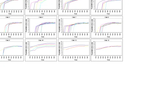
clarity we will show only the graphs for the top 75. Figure 1 shows the evolution over time
of the log-population of the cities in each convergence club (we show the log-population
because by de nition the test is performed with log-variables). Our analysis focuses on
these results. Figure 2 shows the evolution of the top 75 cities, and demonstrates that it is
dif cult to deduce any speci c type of pattern. However, some of the groups represented in
the remainder of the graphs show a sequential pattern, especially in the entry of new cities.
These new cities appear later in the sample, but grow at a faster rate than do the rest of
the cities in their club until they reach similar growth rates to the pre-existing cities.22 It
is surprising that in almost all convergence clubs (groups of cities that converge in growth
rates identi ed by the cluster procedure), the cities do not appear in the sample at the same
time, but rather sequentially. This behavior is consistent with a pattern of sequential city
growth, at least within groups.
20In fact, with the largest cities in 2000 we nd only four convergence clubs, because all of them are cities
characterized by high growth rates. The results are available from the authors on request.
21Altogether, 31 cities (20.7%) of the top 150 cities in 2000 are not in the top 150 cities in 1900. The
differences are greater still in the top 75 and 100, because there are 36 different cities (48% and 36% of the sample, respectively).
22Some of the graphs are similar to Figure 4 (a) in Henderson and Venables (2009), obtained by simulations
The algorithm classi es cities into 12 groups (convergence clubs). There are four
re-maining cities that are not classi ed into any club and for which the convergence
hypothe-sis is rejected. In each group, the estimated coef cient ^1is signi cantly positive, strongly supporting the club classi cation. Furthermore, only one of the estimated coef cients is
signi cantly greater than two (club 2), indicating that the evidence in favor of level
con-vergence is small, while support for conditional concon-vergence within each of the other clubs
is stronger because ^1 < 2. Of the four cities belonging to club 2, three are in the South Region, although the geographical distribution of cities shows no speci c spatial pattern in
any of the groups. Only club 11 consists of cities belonging to the same region (Northeast),
although another common characteristic of these cities is that they are among the oldest.
The cities that have existed since 1790 are classi ed into groups 10 to 12, indicating that
while they present a different growth pattern from the cities that appeared later, they also
differ from each other.
It should be noted that of the 12 clubs, only clubs 1 and 2 correspond to cities that
rise in the ranking (on average) from 1900 to 2000. The cities within the other clubs lose
positions in the ranking (on average), especially those in clubs 7, 9 and 12, con rming
our idea that our sample captures more heterogeneous behaviors than does the sample of
“winning” cities in 2000, especially because we also include “failing” cities that performed
poorly in terms of growth over the entire time interval.
5
Discussion
Thus far, we found mixed evidence regarding city growth in the long-term. First, we
can-not reject the random growth (unit root) hypothesis for most of the proposed speci cations,
against the alternative hypothesis of convergence (mean reversion). However, we nd
evi-dence of high mobility when we model growth as a rst-order Markov process; this
mobil-ity is consistent with the results of other studies that consider the same 1790–2000 period
supporting conditional convergence in city growth rates within convergence clubs, which
we can interpret as “local” mean-reverting behaviors. We interpret the high mobility and
the results of clustering analysis as signs of a sequential city growth pattern.
These results raise two questions: rst, whether these different empirical results are
compatible and, second, whether the city size distribution has evolved according to the
random growth pattern (if Zipf's law holds) or whether, on the contrary, the trend has been
convergence among cities.
The rst question asks whether a random growth result is compatible with a degree of
convergence in the evolution of city growth rates; in other words, whether a unit root is
compatible with some kind of mean-reverting component. Gabaix and Ioannides (2004)
answer this question by putting forward what they call “deviations from Gibrat's Law
(ran-dom growth) that do not affect the distribution,” starting from:
lnSit lnSit 1 = (Xit; t) + it, (8)
where Xit is a possibly time-varying vector of characteristics of city i; (Xit; t) is the expectation of city i's growth rate as a function of economic conditions at timet; and it
is white noise. In the simplest speci cation, itis independently and identically distributed
over time (this means that it has a zero mean and a constant variance that is uncorrelated
with isfort 6=s) and (Xit; t)is constant.
Gabaix and Ioannides (2004) consider two types of deviations, relaxing both
assump-tions. Rossi-Hansberg and Wright (2007) discuss the economic interpretations of
devia-tions from Zipf's and Gibrat's laws. We are interested in the consequences of relaxing the
assumption of an i.i.d. it, assuming constant (Xit; t) = . In its place, the following stochastic structure is assumed: it =bit+ it it 1, wherebitis i.i.d. and it follows a stationary process. Replacing in (8) they obtain:
lnSit lnSi0 = t+
t
X
s=1
The termPts=1bisgives a unit root in the growth process, while the term itcan have any stationarity. According to Gabaix and Ioannides (2004), this means that “for Zipf's law
to hold, the city evolution process can contain a mean reversion component, as long as
it contains a non-zero unit root component.” Therefore, our mixed empirical evidence is
not contradictory, but rather compatible. In addition, our conclusion leads us directly to
our second question, the behavior of city size distribution over the 1790–2000 period (and
whether Zipf's law holds).
Let us denote S as the size (population) and R as its corresponding rank (1 for the
largest, 2 for the second largest and so on). A power law (Pareto distribution) links city
size and rank as follows: R(S) = AS a. This expression has been used extensively in urban economics to study city size distribution (see, for example, Eeckhout (2004) and
Ioannides and Overman (2003) for the US case). It is usually speci ed and estimated in its
logarithmic version:
lnR=b alnS+ , (10)
where is the error term andb andaare the parameters that characterize the distribution.
The latter is known as the Pareto exponent, and Zipf's law is considered to hold when
a = 1. This means that when ordered from largest to smallest, the size of the second city is half that of the rst one, the size of the third is a third of the rst one and so on. The
greater the coef cient, the more homogeneous are the city sizes. In addition, an increase
in the coef cient over time would mean a process of convergence in city sizes. Similarly,
the smaller the coef cient, the less homogeneous are city sizes, and a decreasing evolution
would mean a process of divergence.
Gabaix and Ibragimov (2011) propose specifying Equation (10) by subtracting 1=2
from the rank to obtain an unbiased estimation ofa:
ln R 1
2 =b alnS+ . (11)
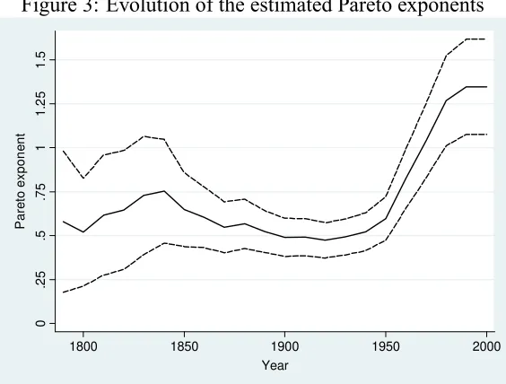
dur-ing the 1790–2000 period. Figure 3 shows the results.23 We estimated using all the cities
available in each decade (from 16 in 1790 to 190 in 2000). The results show that the
distrib-ution remained stable until 1950, so the entry of new cities did not have a signi cant effect,
although the estimated coef cients are less than one, indicating a high degree of inequality
among city sizes. Therefore, during this period the stable evolution of the city size
distrib-ution re ects the random growth process, even though the resulting Pareto exponent of the
distribution is lower than one, rejecting Zipf's law for this group of the largest cities.24
From 1950 the estimated Pareto coef cient grows to reach (and exceed) the value of
one. Note that from 1950 to 2000 only 11 cities enter the sample, so that the evolution of
the exponent reacts only to the city growth process. The increasing trend of the exponents
indicates a process of convergence among cities. We also estimated the Gini coef cients
for each period. The Gini coef cients have the advantage of not imposing a speci c size
distribution (Pareto for rank-size coef cients). The results are similar; from 1790 to 1950,
the Gini coef cient rose from 0.65 to 0.68,25 while in 2000 it was 0.50. Therefore, during
this period the evolution of the distribution clearly corresponds to a convergence phase. The
explanation for this convergence process is well known in the literature (post-war
subur-banization). During the second half of the twentieth century, mid-sized and small American
cities grew much more than did the largest cities in the same metropolitan areas.26 Glaeser
et al. (2011) claim that some of the impact of sprawl and the role that the automobile played
in dispersing the American population can explain some of these patterns. The effect that
we capture from this process is that the cities of the upper-tail distribution became more
homogeneous in size because of the larger growth of mid-sized cities, thereby bringing
them closer to the largest ones.
23The Pareto exponent is estimated using Gabaix and Ibragimov's Rank-1=2estimator. Dashed lines rep-resent the standard errors calculated applying Gabaix and Ioannides's (2004) corrected standard errors: GI s.e.= ^a (2=N)1=2, whereN is the sample size.
24Except in 1830 and 1840, for which the con dence intervals indicate that we cannot reject the fact that
the coef cient is signi cantly different from one.
25However, the evolution of the Gini coef cient is not as stable as that of the Pareto exponent, because
within this period it does re ect changes in the inequality of the distribution in some decades.
26Several works have studied the causes of this process. For example, Margo (1992) examines the role of
6
Conclusions
In this paper, we study the growth pattern of the system of cities in the United States from its
origin. We obtain several conclusions. First, we nd evidence supporting random growth in
American cities during the 1790–2000 period, indicating that the growth rate does not
de-pend on initial size. Second, we nd evidence of high intra-distribution mobility when we
consider growth as a rst-order Markov process. Third, using a cluster procedure we nd
evidence in favor of the conditional convergence of city growth rates within convergence
clubs, allowing us to conclude that “local” mean-reverting behaviors exist. Our results lend
support to recent theories of sequential city growth.
References
Baltagi, B. H., (2008). Econometric Analysis of Panel Data. Wiley: Chichester, Fourth
Edition.
Banerjee, A., M. Massimiliano, and C. Osbat, (2005). Testing for PPP: should we use
panel methods? Empirical Economics, 30: 77–91.
Batty, M., (2006). Rank clocks. Nature, Vol. 444, 30 November 2006, 592–596.
Beeson, P.E., D. N. DeJong, and W. Troesken, (2001). Population Growth in US
Coun-ties, 1840-1990. Regional Science and Urban Economics, 31: 669–699.
Black, D., and V. Henderson, (1999). Spatial Evolution of Population and Industry in
the United States. The American Economic Review, Vol. 89(2), Papers and Proceedings of
the One Hundred Eleventh Annual Meeting of the American Economic Association (May,
1999), 321–327.
Black, D., and V. Henderson, (2003). Urban evolution in the USA. Journal of Economic
Geography, Vol. 3(4): 343–372.
shocks: the evolution of the German city size distribution 1925–1999. Regional Science
and Urban Economics 38: 330–347.
Breitung, J., (2000). The Local Power of Some Unit Root Tests for Panel Data.
Ad-vances in Econometrics, 15: 161–177.
Bridenbaugh, C., (1938). Cities in the Wilderness. The Ronald Press.
Canova, F., (2004). Testing for convergence clubs in income per capita: a predictive
density approach. International Economic Review, 45: 49–77.
Champernowne, D., (1953). A model of income distribution. Economic Journal, LXIII:
318–351.
Cheshire, P. C., and S. Magrini, (2006). Population Growth in European Cities: Weather
Matters – but only Nationally. Regional Studies, 40(1): 23–37.
Clark, J. S., and J. C. Stabler, (1991). Gibrat's Law and the Growth of Canadian Cities.
Urban Studies, 28(4): 635–639.
Córdoba, J. C., (2008). A generalized Gibrat's law. International Economic Review,
Vol. 49(4): 1463–1468.
Cuberes, D., (2009). A Model of Sequential City Growth. The B.E. Journal of
Macro-economics: Vol. 9: Iss. 1 (Contributions), Article 18.
Cuberes, D., (2011). Sequential City Growth: Empirical Evidence. Journal of Urban
Economics, 69: 229–239.
Davis, D. R., and D. E. Weinstein, (2002). Bones, bombs, and break points: the
geog-raphy of economic activity. American Economic Review, 92(5): 1269–1289.
Dickey, D. A., and W. A. Fuller, (1979). Distributions of the Estimators for
Autoregres-sive Time Series with a Unit Root. Journal of American Statistical Association, 74(366):
427–481.
distribution. Included in Huriot, J. M. and J. F. Thisse (Eds.), The economics of cities.
Cambridge University Press, Cambridge, pp. 217–260.
Dobkins, L. H., and Y. M. Ioannides, (2001). Spatial interactions among U.S. cities:
1900–1990. Regional Science and Urban Economics 31: 701–731.
Duranton, G., (2007). Urban Evolutions: The Fast, the Slow, and the Still. American
Economic Review, 97(1): 197–221.
Durlauf, S. N., and P. A. Johnson, (1995). Multiple regimes and cross-country growth
behavior. Journal of Applied Econometrics, 10: 365–384.
Eaton, J., and Z. Eckstein, (1997). Cities and Growth: Theory and Evidence from
France and Japan. Regional Science and Urban Economics, 27(4 –5): 443–474.
Eeckhout, J., (2004). Gibrat's Law for (All) Cities. American Economic Review, 94(5):
1429–1451.
Eeckhout, J., (2009). Gibrat's Law for (all) Cities: Reply. American Economic Review,
99(4): 1676–1683.
Ellison, G., and E. L. Glaeser, (1999). The geographic concentration of industry: Does
natural advantage explain agglomeration? American Economic, Review Papers and
Pro-ceedings, 89(2): 311–316.
Gabaix, X., (1999). Zipf's law for cities: An explanation. Quarterly Journal of
Eco-nomics, 114(3): 739–767.
Gabaix, X., and R. Ibragimov, (2011). Rank-1/2: A simple way to improve the OLS
estimation of tail exponents. Journal of Business & Economic Statistics, 29(1): 24–39.
Gabaix, X., and Y. M. Ioannides, (2004). The evolution of city size distributions.
Hand-book of urban and regional economics, Vol. 4, J. V. Henderson and J. F. Thisse, eds.
Ams-terdam: Elsevier Science, North-Holland, pp. 2341–2378.
Galor, O., (1996). Convergence? Inferences from Theoretical Models. The Economic
Garmestani, A. S., C. R. Allen, and K. M. Bessey, (2005). Time-series Analysis of
Clusters in City Size Distributions. Urban Studies, Vol. 42(9): 1507–1515.
Garmestani, A. S., C. R. Allen, and C. M. Gallagher, (2008). Power laws,
discontinu-ities and regional city size distributions. Journal of Economic Behavior & Organization,
68: 209–216.
Giesen, K., A. Zimmermann, and J. Suedekum, (2010). The size distribution across all
cities – double Pareto lognormal strikes. Journal of Urban Economics, 68: 129–137.
Glaeser, E. L., and J. Gyourko, (2005). Urban Decline and Durable Housing. Journal
of Political Economy, 113(2): 345–375.
Glaeser, E. L., G. A. M. Ponzetto, and K. Tobio, (2011). Cities, Skills, and Regional
Change. Forthcoming in Regional Studies.
González-Val, R., (2010). The Evolution of the US City Size Distribution from a
Long-run Perspective (1900–2000). Journal of Regional Science, 50(5): 952–972.
González-Val, R., L. Lanaspa, and F. Sanz, (2010). New Evidence on Gibrat's Law for
Cities. MPRA Working Paper No. 26924.
Hamilton, J. D., (1994). Time Series Analysis. Princeton, NJ: Princeton University
Press.
Henderson, J. V., and A. Venables, (2009). The Dynamics of City Formation. Review
of Economic Dynamics, 12: 233–254.
Henderson, J. V., and H. G. Wang, (2007). Urbanization and city growth: The role of
institutions. Regional Science and Urban Economics, 37(3): 283–313.
Im, K. S., M. H. Pesaran, and Y. Shin, (2003). Testing for Unit Roots in Heterogeneous
Panels. Journal of Econometrics, 115: 53–74.
Ioannides, Y. M. and H. G. Overman, (2003). Zipf's law for cities: an empirical
Kim, S., (2000). Urban development in the United States. Southern Economic Journal
66, 855–880.
Kim, S., and R. A. Margo, (2004). Historical perspectives on U.S. Economic
Geogra-phy. Handbook of urban and regional economics, vol. 4, J. V. Henderson and J. F. Thisse,
eds. Amsterdam: Elsevier Science, North-Holland, Chapter 66, pp. 2982–3019.
Lanaspa-Santolaria, L. F., A. Montañes, L. I. Olloqui-Cuartero, and F. Sanz-Gracia,
(2002). The Phenomenon of Regional Inversion in the US manufacturing sector. Papers in
Regional Science, 81(4): 461–482
Lanaspa, L. F., F. Pueyo, and F. Sanz, (2011). Urban dynamics during the twentieth
century. A tale of ve European countries. Mimeo, Universidad de Zaragoza.
Levin, A., C.-F. Lin, and C.-S. J. Chu, (2002). Unit Root Tests in Panel Data:
Asymp-totic and Finite Sample Properties. Journal of Econometrics, 108: 1–24.
Levy, M., (2009). Gibrat's Law for (all) Cities: A Comment. American Economic
Review, 99(4): 1672–1675.
Margo, R. A., (1992). Explaining the Postwar Suburbanization of Population in the
United States: The Role of income. Journal of Urban Economics, 31: 301–310.
Melo, P. C., D. J. Graham, and R. B. Noland, (2009). A Meta-analysis of Estimates of
Urban Agglomeration Economies. Regional Science and Urban Economics, 39: 332–342.
Michaels, G., F. Rauch, and S. J. Redding, (2010). Urbanization and Structural
Trans-formation. Unpublished manuscript, London School of Economics.
Overman, H. G., and Y. M. Ioannides, (2001). Cross-Sectional Evolution of the U.S.
City Size Distribution. Journal of Urban Economics 49, 543–566.
Quah, D., (1993). Empirical cross-section dynamics in economic growth. European
Economic Review, 31: 426–434.
Pesaran, M. H., (2007). A simple panel unit root test in the presence of cross-section
Phillips, P. C. B., and D. Sul, (2007). Transition Modeling and Econometric
Conver-gence Tests. Econometrica, Vol. 75, 1771–1855.
Phillips, P. C. B., and D. Sul, (2009). Economic Transition and Growth. Journal of
Applied Econometrics, 24, 1153–1185.
Resende, M., (2004). Gibrat's Law and the Growth of Cities in Brazil: A Panel Data
Investigation. Urban Studies, Vol. 41(8): 1537–1549.
Rossi-Hansberg, E., and M. L. J. Wright, (2007). Urban structure and growth. Review
of Economic Studies, 74: 597–624.
Rozenfeld, H. D., D. Rybski, X. Gabaix, and H. A. Makse, (2011). The Area and
Popu-lation of Cities: New Insights from a Different Perspective on Cities. American Economic
Review, forthcoming.
Said, S. E., and D. A. Dickey, (1984). Testing for Unit Roots in Autoregressive-Moving
Average Models of Unknown Order. Biometrika, 71(3): 599–607.
Sharma, S., (2003). Persistence and Stability in City Growth. Journal of Urban
Eco-nomics 53: 300–320.
Simon, H., (1955). On a class of skew distribution functions. Biometrika, 42: 425–440.
Soo, K.T., (2007) Zipf's Law and Urban Growth in Malaysia. Urban Studies 44(1):
1–14
U.S. Census Bureau, (2004). 2000 Census of Population and Housing, Population and
Housing Unit Counts PHC-3-1, United States Summary. Washington, DC. Available at:
http://www.census.gov/prod/cen2000/phc3-us-pt1.pdf.
Vining, D. R., (1976). Autocorrelated Growth Rates and the Pareto Law: A Further
Table 1: NUMBER OF CITIES AND DESCRIPTIVESTATISTICS BYYEAR
Year Cities Mean Standard deviation Minimum Maximum US urban population (UP) % of UP
1790 16 8,746.50 13,313.13 200 49,401 201,655 69.40%
1800 22 10,255.00 18,565.84 81 79,216 322,371 69.98%
1810 25 14,278.04 26,052.55 383 119,734 525,459 67.93%
1820 28 16,832.07 31,499.38 606 152,056 693,255 67.98%
1830 36 20,631.19 43,079.73 877 242,278 1,127,247 65.89%
1840 50 24,502.46 58,753.40 1,222 391,114 1,845,055 66.40%
1850 73 30,220.67 85,663.40 415 696,115 3,574,496 61.72%
1860 94 44,193.24 136,697.40 175 1,174,779 6,216,518 66.82%
1870 110 55,417.75 160,729.66 155 1,478,103 9,902,361 61.56%
1880 125 65,037.17 197,482.93 556 1,911,698 14,129,735 57.54%
1890 149 77,799.07 232,080.75 273 2,507,414 22,106,265 52.44%
1900 157 108,432.39 329,863.51 202 3,437,202 30,214,832 56.34%
1910 165 142,935.56 433,335.63 297 4,766,883 42,064,001 56.07%
1920 171 176,340.04 509,938.16 326 5,620,048 54,253,282 55.58%
1930 179 211,572.36 614,701.55 515 6,930,446 69,160,599 54.76%
1940 179 224,762.88 651,013.99 582 7,454,995 74,705,338 53.85%
1950 179 260,994.59 695,986.21 727 7,891,957 96,846,817 48.24%
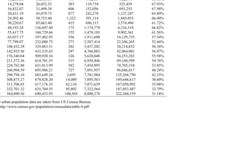
1960 182 290,794.10 683,649.24 3,695 7,781,984 125,268,750 42.25% 1970 187 308,875.27 679,828.20 14,089 7,895,563 149,646,617 38.60% 1980 188 311,706.85 617,176.35 62,134 7,071,639 167,050,992 35.08% 1990 190 332,701.32 635,704.55 95,802 7,322,564 187,053,487 33.79% 2000 190 364,890.56 690,433.95 100,565 8,008,278 222,360,539 31.18%
Note:US urban population data are taken from US Census Bureau. Source: http://www.census.gov/population/censusdata/table-4.pdf
Table 2: PANEL UNIT ROOT TESTS, PESARAN'S CADFSTATISTIC Panel A: 1790-1900. Year of reference for Top cities: 1860
Augmenting lag (1) Augmenting lags (2) Augmenting lags (3) Sample Size Constant Constant & trend Constant Constant & trend Constant Constant & trend
Top 10 4.448 (1.000) 4.522 (1.000) 10.877 (1.000) 8.882 (1.000) 10.877 (1.000) 8.882 (1.000) Top 75 18.021 (1.000) 15.331 (1.000)
Panel B: 1900-2000. Year of reference for Top cities: 1900
Augmenting lag (1) Augmenting lags (2) Augmenting lags (3) Sample Size Constant Constant & trend Constant Constant & trend Constant Constant & trend
Top 10 2.673 (0.996) 0.374 (0.646) 12.533 (1.000) 11.253 (1.000) 12.533 (1.000) 11.253 (1.000) Top 75 5.152 (1.000) 1.049 (0.853) 34.011 (1.000) 30.349 (1.000) 34.011 (1.000) 30.349 (1.000) Top 100 -0.799 (0.212) 2.250 (0.988) 39.273 (1.000) 35.044 (1.000) 39.273 (1.000) 35.044 (1.000) Top 150 -5.100 (0.000) 2.612 (0.995) 48.540 (1.000) 43.583 (1.000) 48.540 (1.000) 43.583 (1.000) Panel C: 1790-2000. Year of reference for Top cities: 1900
Augmenting lag (1) Augmenting lags (2) Augmenting lags (3) Sample Size Constant Constant & trend Constant Constant & trend Constant Constant & trend
Top 10 -4.110 (0.000) -1.593 (0.056) -1.394 (0.082) -1.626 (0.052) -3.212 (0.001) -1.752 (0.040) Top 75 -8.251 (0.000) -8.067 (0.000) -3.507 (0.000) -0.805 (0.210) 4.165 (1.000) 12.598 (1.000) Top 100 -5.489 (0.000) -5.468 (0.000) -0.071 (0.472) 1.575 (0.942) 10.535 (1.000) 18.987 (1.000) Top 150 -7.645 (0.000) -1.397 (0.081) -2.471 (0.007) 9.946 (1.000) 20.622 (1.000) 28.679 (1.000)
Note:Pesaran's (2007)Z[t]test-statistic (p-value). Sample may not contain gaps; therefore, the eight gaps in the sample were lled using values calculated by linear interpolation.
Table 3: AVERAGE10-YEAR TRANSITION MATRICES
Panel A: 1790-1900 Panel B: 1900-2000 Panel C: 1790-2000
Sample Size: 75 Sample Size: 75 Sample Size: 75
1 2 1 0.7 0.4 1 2 1 0.7 0.4 1 2 1 0.7 0.4
1 0.933 0.067 0 0 0 1 0.922 0.078 0 0 0 1 0.928 0.072 0 0 0
2 0.082 0.755 0.163 0 0 2 0.033 0.856 0.111 0 0 2 0.050 0.820 0.130 0 0
1 0 0.279 0.512 0.209 0 1 0 0.112 0.747 0.141 0 1 0 0.162 0.676 0.162 0
0.7 0 0.011 0.080 0.670 0.239 0.7 0 0.005 0.076 0.839 0.080 0.7 0 0.006 0.077 0.792 0.125
0.4 0 0.004 0.010 0.086 0.900 0.4 0 0 0.013 0.134 0.853 0.4 0 0.002 0.012 0.106 0.880
Xt 0 0 0 0 0.05751 Xt 0 0 0 0.00135 0.07143 Xt 0 0 0 0.00073 0.06506
Zt 0 0.00160 0.00160 0.00320 0.14537 Zt 0 0 0 0.00674 0.06604 Zt 0 0.00073 0.00073 0.00512 0.10234
Sample Size: 100 Sample Size: 100 Sample Size: 100
1 2 1 0.7 0.4 1 2 1 0.7 0.4 1 2 1 0.7 0.4
1 0.918 0.082 0 0 0 1 0.913 0.087 0 0 0 1 0.915 0.085 0 0 0
2 0.102 0.780 0.102 0.016 0 2 0.056 0.839 0.105 0 0 2 0.071 0.820 0.104 0.005 0
1 0 0.102 0.592 0.306 0 1 0 0.118 0.756 0.126 0 1 0 0.114 0.710 0.176 0
0.7 0 0.041 0.082 0.653 0.224 0.7 0 0.009 0.101 0.780 0.110 0.7 0 0.018 0.095 0.742 0.145
0.4 0 0.003 0.003 0.087 0.907 0.4 0 0 0.011 0.122 0.867 0.4 0 0.001 0.007 0.105 0.887
Xt 0 0 0 0 0.02307 Xt 0 0 0 0 0.06949 Xt 0 0 0 0 0.04971
Zt 0 0.00136 0.00136 0.00407 0.13026 Zt 0 0 0 0.00302 0.06647 Zt 0 0.00058 0.00058 0.00347 0.09364
Sample Size: 150 Sample Size: 150 Sample Size: 150
1 2 1 0.7 0.4 1 2 1 0.7 0.4 1 2 1 0.7 0.4
1 0.921 0.079 0 0 0 1 0.898 0.102 0 0 0 1 0.908 0.092 0 0 0
2 0.143 0.661 0.196 0 0 2 0.068 0.837 0.095 0 0 2 0.085 0.797 0.118 0 0
1 0 0.141 0.684 0.175 0 1 0.006 0.116 0.749 0.129 0 1 0.005 0.123 0.731 0.141 0
0.7 0 0.037 0.111 0.667 0.185 0.7 0 0.018 0.078 0.806 0.098 0.7 0 0.023 0.086 0.771 0.120
0.4 0 0 0.002 0.084 0.914 0.4 0 0.002 0.003 0.125 0.870 0.4 0 0.001 0.003 0.109 0.887
Xt 0 0 0 0 0.00407 Xt 0 0 0 0 0.03928 Xt 0 0 0 0 0.02608
Zt 0 0.00114 0.00114 0.00457 0.14400 Zt 0 0 0 0.00333 0.03595 Zt 0 0.00042 0.00042 0.00379 0.07783
Table 4: CONVERGENCE CLUBS, 1790-2000
Club 1 (t-statistic) Club 1(t-statistic) Club 1 (t-statistic) 1 [7] 0.105 (0.146) 1 [12] 0.744 (2.386) 1 [26] 1.217 (6.979) 2 [4] 2.507 (3.844) 2 [7] 0.671 (4.686) 2 [17] 0.254 (3.720) 3 [6] 0.893 (2.326) 3 [6] 0.893 (2.326) 3 [9] 0.225 (2.674) 4 [5] 0.256 (3.225) 4 [7] 0.142 (0.910) 4 [15] 0.141 (1.634) 5 [6] 0.294 (1.885) 5 [12] 0.560 (2.119) 5 [20] 0.400 (1.462) 6 [8] 0.435 (5.784) 6 [12] 0.010 (0.087) 6 [23] 0.064 (0.502) 7 [14] 0.224 (2.389) 7 [18] 0.370 (4.367) 7 [21] 0.539 (4.215) 8 [6] 1.970 (1.188) 8 [6] 1.970 (1.188) 8 [3] 2.405 (2.303) 9 [4] 0.353 (0.985) 9 [5] 0.700 (2.794) 9 [6] 0.011 (0.396) 10 [5] 0.224 (4.673) 10 [5] 0.224 (4.673) 10 [3] 0.842 (6.385) 11 [3] 0.842 (6.385) 11 [3] 0.842 (6.385) 11 [3] 0.347 (0.711) 12 [3] 0.347 (0.711) 12 [3] 0.347 (0.711)
Sample Size: Top 75 Sample Size: Top 100 Sample Size: Top 150
Note: The numbers in brackets are the number of cities.Top cities are de ned according to
Figure 1: Cities' log population evolution, Top 75, 1790–2000: Convergence clubs
Figure 2: Cities' log population evolution, Top 75, 1790–2000 All cities 0 2 4 6 8 10 12 14 16 18 17 90 18 10 18 30 18 50 18 70 189 0 19 10 19 30 195 0 197 0 19 90 Year P opu lat io n (l n scal e)
Figure 3: Evolution of the estimated Pareto exponents
0 .25 .5 .75 1 1 .25 1 .5 Pare to expon e nt
[image:36.612.158.440.310.524.2]Appendix: Cities within clubs
CITIES WITHIN CLUBS
Rank in 1900 First year in the sample Name Club (Sample Size: Top 75) Club (Sample Size: Top 100) Club (Sample Size: Top 150)
1 1790 New York 10 10 9
2 1840 Chicago
3 1790 Philadelphia 10 10 9
4 1830 St. Louis 2 2 2
5 1790 Boston 11 11 10
6 1790 Baltimore 10 10 9
7 1820 Cleveland 1 1 1
8 1810 Buffalo 3 3 3
9 1850 San Francisco 1 1 1
10 1810 Cincinnati 4 4 4
11 1800 Pittsburgh 3 3 3
12 1810 New Orleans 3 3 3
13 1820 Detroit 1 1 1
14 1840 Milwaukee 1 1 1
15 1800 Washington 2 2 2
16 1830 Newark 3 3 3
17 1840 Jersey 8 8 7
18 1790 Louisville 10 10 9
19 1860 Minneapolis 6 6 6
20 1790 Providence
21 1840 Indianapolis 3 3 3
22 1860 Kansas 5 5 5
23 1850 St. Paul 7 7 6
24 1830 Rochester 8 8 7
25 1860 Denver 5 5 5
26 1840 Toledo 6 6 6
27 1830 Columbus 3 3 3
28 1790 Worcester 11 11 10
29 1850 Syracuse 9 9 7
30 1790 New Haven
31 1840 Paterson 7 7 7
32 1860 Omaha 5 5 5
33 1850 Los Angeles 1 1 1
34 1850 Memphis 4 4 4
35 1830 Lowell 7 7 7
36 1790 Cambridge 12 12 11
37 1860 Portland 4 4 4
38 1850 Atlanta 6 6 6
39 1850 Grand Rapids 6 6 6
40 1810 Dayton 8 8 6
41 1790 Richmond 12 12 11
42 1800 Nashville-Davidson 1 1 1
43 1870 Seattle 5 5 5
44 1790 Hartford
45 1840 Bridgeport 8 8 7
46 1860 Oakland 6 6 6
47 1860 Des Moines 7 7 7
48 1790 Spring eld 11 11 10
49 1850 Evansville 9 9 7
50 1790 Manchester 10 10 9
51 1840 Peoria 7 7 7
52 1800 Savannah 7 7 7